Why Does My Resampled Land Cover Have Classes That Should Not Be There?

On this page

Problem statement

You resample a land cover raster to a coarser grid, or reproject it, and the result contains codes like 13, 27 or 64 that are not in the legend. Or worse, it contains plenty of a real class that was rare before. The cause is the resampling method. Bilinear, cubic and average resampling compute weighted means of the neighbouring values, which for temperatures is right and for class codes is meaningless: the mean of grassland (71) and cultivated crops (82) is 76.5, and many blends of evergreen forest (42) with higher-coded neighbours come out as 43, mixed forest, which then appears where no mixed forest was.

This page resamples NLCD 2021 for Williamson County, Texas, from 30 m to 300 m with four methods and measures what each does to the classes and their areas.

Quick answer

Use nearest neighbour (or mode) for categorical rasters, never bilinear, cubic or average. Check for invented codes after any resampling:

def resample(method):
    out = np.zeros(SHAPE_300, np.uint8)
    reproject(LC, out, src_transform=TRANSFORM, src_crs="EPSG:5070", dst_transform=T300, dst_crs="EPSG:5070",
              resampling=getattr(Resampling, method), src_nodata=0, dst_nodata=0)
    return out

R = {m: resample(m) for m in ("nearest", "bilinear", "average", "mode")}
for m, r in R.items():
    invented = sorted({int(v) for v in np.unique(r)} - CODES - {0})
    print(f"{m:8s}: {len(invented):2d} codes not in NLCD, on {np.isin(r, invented).sum() / (r > 0).sum():.0%} of pixels")

nearest :  0 codes not in NLCD, on 0% of pixels
bilinear: 66 codes not in NLCD, on 76% of pixels
average : 66 codes not in NLCD, on 69% of pixels
mode    :  0 codes not in NLCD, on 0% of pixels

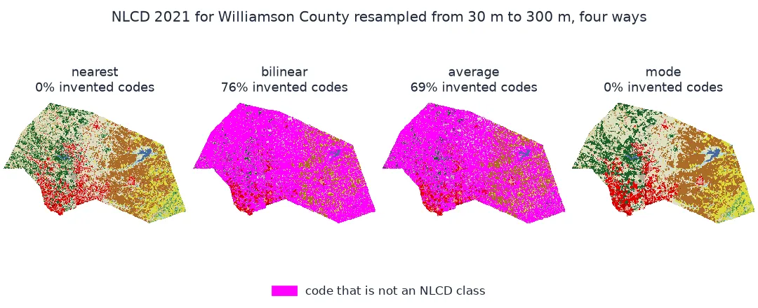
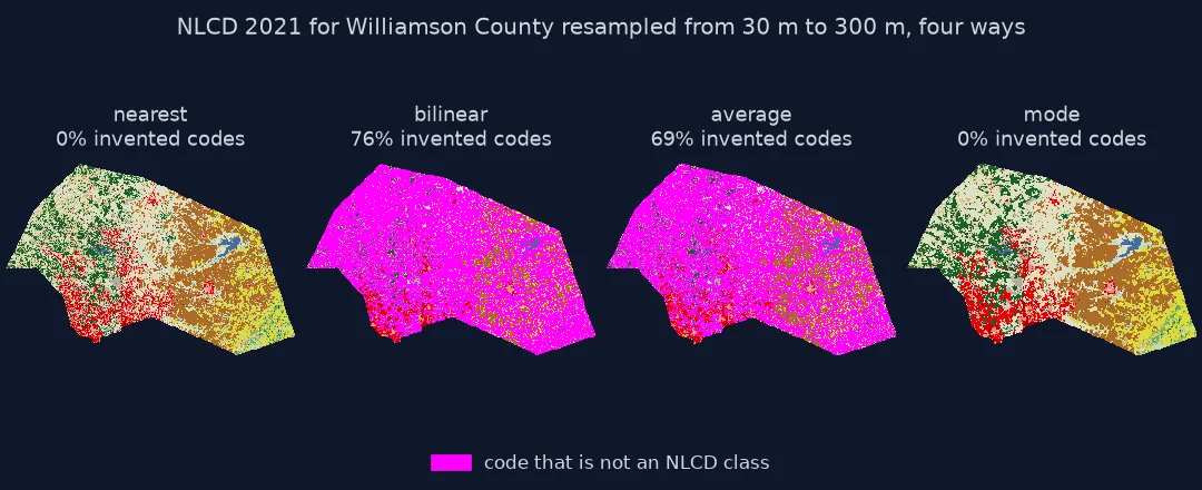
Four maps of Williamson County land cover at 300 metres: nearest neighbour and mode look like the original classes, while bilinear and average are mostly magenta, marking codes that are not NLCD classes, on 76 and 69 percent of pixels. — The same raster resampled four ways. Averaging methods fill most of the map with codes that are not classes.

Spot invented codes, compare nearest and mode, use fractions

1. See which invented codes look real

Some averaged values land exactly on a real class code, and those are the dangerous ones, because no check for unknown codes catches them:

area = lambda r, k: (r == k).sum() * 300 * 300 / 1e6
t = pd.DataFrame({"30 m": {k: (LC == k).sum() * 900 / 1e6 for k in sorted(CODES)}})
for m in R:
    t[m] = {k: area(R[m], k) for k in sorted(CODES)}
t.index = [f"{k} {NLCD_CLASSES[k]}" for k in t.index]
print(t.round(1).to_string())

                         30 m  nearest  bilinear  average   mode
11 Open water            32.4     32.0       7.8     11.8   28.4
21 Developed, open      170.3    175.0       1.0      2.9   59.0
22 Developed, low       134.8    135.0      23.6     42.0   73.3
23 Developed, medium    165.2    163.1      60.6     82.5  216.1
24 Developed, high       53.0     51.7      42.8     39.7   39.8
31 Barren                33.3     33.9      22.1     23.9   31.9
41 Deciduous forest     112.4    116.2      29.1     31.9   50.5
42 Evergreen forest     314.3    315.6      44.8     60.1  380.5
43 Mixed forest           8.8      7.9      44.3     46.7    3.2
52 Shrub/scrub          167.0    161.8      40.3     39.1  109.8
71 Grassland            757.8    760.0      80.7    117.1  899.5
81 Pasture/hay          272.2    270.1     127.4    135.4  312.4
82 Cultivated crops     639.7    639.7     184.0    277.6  707.8
90 Woody wetlands        61.7     60.6       0.4      1.8   53.3
95 Herbaceous wetlands    3.4      3.2       0.0      0.0    0.5

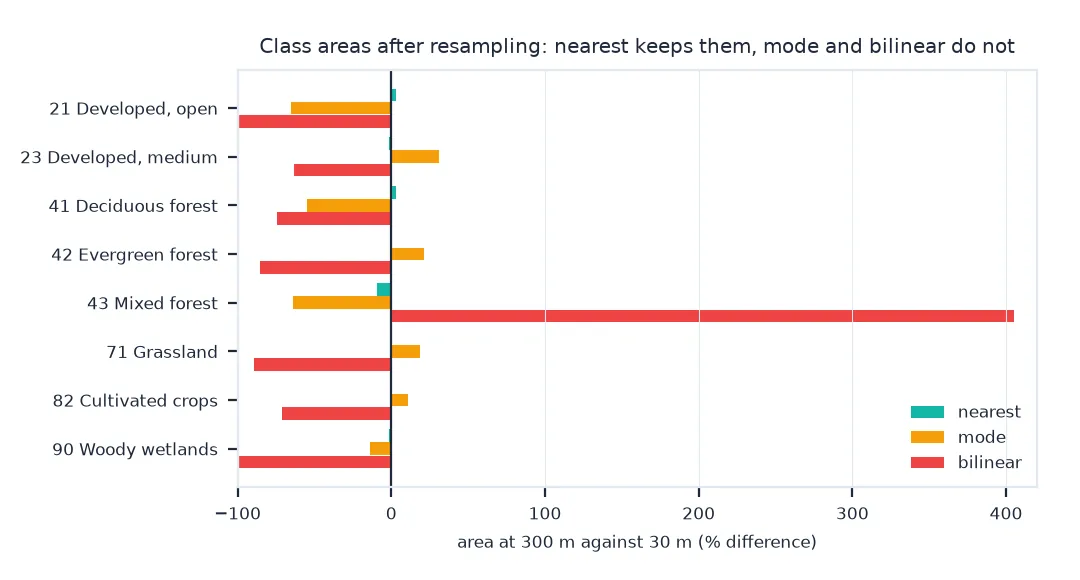
Mixed forest (43) is the clearest case: bilinear and average resampling multiply it about fivefold, by averaging deciduous (41), evergreen (42) and other neighbours into its code. Open water and wetlands nearly vanish, because their codes are far from their neighbours'.

2. Compare nearest and mode

Nearest neighbour takes the class at each output cell's centre; mode takes the most common class among the input cells. Both keep valid codes, but they bias area differently:

err = t[["nearest", "mode"]].sub(t["30 m"], axis=0)
print(f"largest area error, nearest: {err['nearest'].abs().max():.1f} km²; mode: {err['mode'].abs().max():.1f} km²")
print("mode: dominant classes grow, scattered ones shrink:")
print(err["mode"].sort_values().iloc[[0, 1, -2, -1]].round(1).to_string())

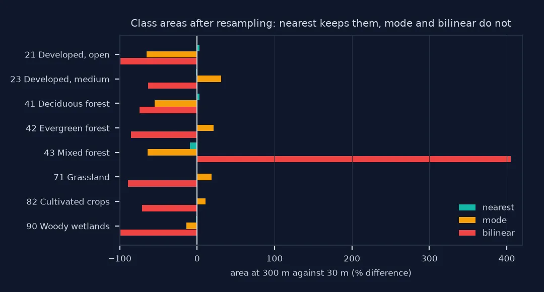
largest area error, nearest: 5.2 km²; mode: 141.7 km²
mode: dominant classes grow, scattered ones shrink:
21 Developed, open    -111.2
41 Deciduous forest    -61.9
82 Cultivated crops     68.0
71 Grassland           141.7

Bar chart of the change in class area after resampling to 300 metres: nearest neighbour within a few percent for every class; mode shrinks developed open space by about 65 percent and deciduous forest by about 55 while growing grassland and evergreen forest by about 20; bilinear removes most of nearly every class but multiplies mixed forest about fivefold. — Class areas after resampling, against the 30 m truth.

3. Aggregate to fractions when area matters

If the coarse grid feeds an analysis of amounts, keep every class as a fraction of each coarse cell instead of choosing one class:

block = LC[:SHAPE_300[0] * 10, :SHAPE_300[1] * 10].reshape(SHAPE_300[0], 10, SHAPE_300[1], 10)
frac = {k: (block == k).mean(axis=(1, 3)) for k in sorted(CODES)}
dev_km2 = sum(frac[k] for k in (21, 22, 23, 24)).sum() * 300 * 300 / 1e6
dev_true = np.isin(LC[:SHAPE_300[0] * 10, :SHAPE_300[1] * 10], [21, 22, 23, 24]).sum() * 900 / 1e6
print(f"developed area from fractions: {dev_km2:.1f} km²; at 30 m over the same cells: {dev_true:.1f} km²")

developed area from fractions: 523.2 km²; at 30 m over the same cells: 523.2 km²

Fractions preserve area exactly and keep the mixture that one class per cell throws away.

What one coarse cell holds

The data used on this page

NLCD 2021 (30 m) for Williamson County, Texas, from MRLC's WCS, masked to the 2023 Census county outline, and resampled within its own CRS (EPSG:5070) to a 300 m grid aligned with the 30 m one.

import time
from pathlib import Path

import geopandas as gpd
import numpy as np
import pandas as pd
import rasterio
import rasterio.mask
import requests
from rasterio.enums import Resampling
from rasterio.warp import reproject

Path("data").mkdir(exist_ok=True)
if not Path("data/cb_2023_us_county_20m.zip").exists():
    Path("data/cb_2023_us_county_20m.zip").write_bytes(requests.get("https://www2.census.gov/geo/tiger/GENZ2023/shp/cb_2023_us_county_20m.zip", timeout=300).content)
COUNTY = gpd.read_file("data/cb_2023_us_county_20m.zip").query("GEOID == '48491'").to_crs(5070)
path = Path("data/nlcd_2021.tif")
if not path.exists():
    x0, y0, x1, y1 = COUNTY.total_bounds
    for attempt in range(4):
        r = requests.get("https://www.mrlc.gov/geoserver/mrlc_download/wcs", params={"service": "WCS", "version": "2.0.1", "request": "GetCoverage",
                         "coverageId": "mrlc_download__NLCD_2021_Land_Cover_L48", "subset": [f"X({x0},{x1})", f"Y({y0},{y1})"], "format": "image/geotiff"}, timeout=300)
        if r.status_code < 500:
            break
        time.sleep(15 * (attempt + 1))
    r.raise_for_status()
    path.write_bytes(r.content)
with rasterio.open(path) as src:
    lc, TRANSFORM = rasterio.mask.mask(src, COUNTY.geometry, crop=True, nodata=0)
LC = lc[0]
CODES = {int(v) for v in np.unique(LC)} - {0}
SHAPE_300 = (LC.shape[0] // 10, LC.shape[1] // 10)
T300 = TRANSFORM * TRANSFORM.scale(10, 10)
NLCD_CLASSES = {11: "Open water", 21: "Developed, open", 22: "Developed, low", 23: "Developed, medium", 24: "Developed, high",
                31: "Barren", 41: "Deciduous forest", 42: "Evergreen forest", 43: "Mixed forest", 52: "Shrub/scrub", 71: "Grassland",
                81: "Pasture/hay", 82: "Cultivated crops", 90: "Woody wetlands", 95: "Herbaceous wetlands"}
print(f"30 m: {LC.shape[1]} x {LC.shape[0]}; 300 m: {SHAPE_300[1]} x {SHAPE_300[0]}; {len(CODES)} classes present")

30 m: 2845 x 1884; 300 m: 284 x 188; 15 classes present

Example 1: what one coarse cell holds

j, i = np.unravel_index(np.argmax(sum(frac[k] > 0 for k in frac)), SHAPE_300)
print(f"the most mixed 300 m cell holds {sum(frac[k][j, i] > 0 for k in frac)} classes:",
      {NLCD_CLASSES[k]: f"{frac[k][j, i]:.0%}" for k in frac if frac[k][j, i] > 0})
print({m: f"{R[m][j, i]} {NLCD_CLASSES.get(int(R[m][j, i]), '(not a class)')}" for m in R})

the most mixed 300 m cell holds 12 classes: {'Open water': '7%', 'Developed, open': '3%', 'Developed, low': '8%', 'Developed, medium': '4%', 'Deciduous forest': '2%', 'Mixed forest': '5%', 'Shrub/scrub': '5%', 'Grassland': '5%', 'Pasture/hay': '28%', 'Cultivated crops': '10%', 'Woody wetlands': '21%', 'Herbaceous wetlands': '2%'}
{'nearest': '11 Open water', 'bilinear': '64 (not a class)', 'average': '65 (not a class)', 'mode': '81 Pasture/hay'}

Resampling methods interpolate

Resampling methods are interpolators. Bilinear, cubic and average methods assume that values between two pixels lie between their values, which holds for temperature, elevation or reflectance. Class codes are labels with arbitrary numbers, so averaging them produces a number, sometimes a valid code, that no pixel had and no mixture means. That the error can produce a real class is what makes it hard to notice: a histogram shows nothing strange about mixed forest, only too much of it.

Which method for which purpose.

Nearest neighbour and mode are the categorical choices, and they differ in what they lose. Nearest neighbour samples one input pixel per output cell, so class areas stay close to the truth on average while the map gets noisier. Mode keeps the dominant class of each cell, which gives a cleaner map but systematically inflates common classes and erases scattered ones, such as small patches of developed land or streams. When areas matter more than a single label, class fractions per cell are exact.

Defaults, reprojection and overviews

Categorical resampling problems and fixes.

Defaults: gdalwarp uses nearest by default, but many tools (rioxarray.reproject with some settings, xarray.coarsen().mean(), image libraries) average.
Reprojection counts: any reprojection resamples; categorical rasters need Resampling.nearest even when the pixel size stays the same.
Overviews: build overviews of categorical rasters with NEAREST or MODE, or zoomed-out views show invented classes.
Upsampling to a finer grid with nearest is safe; it just repeats pixels.
Fractions: rasterio Resampling.sum on one-hot class layers, or a block reshape as here, gives class fractions.

Internal links

Raster resampling explained — the methods in general
How to reclassify a land cover raster — changing codes deliberately

FAQ

Which resampling method should I use for land cover?

Nearest neighbour, or mode when aggregating to a coarser grid. Never bilinear, cubic or average.

Why does my reprojected land cover have new class values?

The reprojection used an averaging resampling method, which computes means of class codes. Reproject with Resampling.nearest.

What is the difference between nearest and mode resampling?

Nearest takes the class at each output cell's centre; mode takes the most common class in the cell. Mode gives cleaner maps but over-represents dominant classes.

How do I aggregate land cover without losing area?

Compute the fraction of each class in every coarse cell instead of assigning one class.