Why Is My Land Cover Change Map Full of Speckle?

Problem statement

Subtract two land cover maps and the "change" map looks like salt and pepper: thousands of single pixels and tiny clusters scattered everywhere, few of them believable. Most come from the maps disagreeing about pixels on class edges, or about classes that are hard to tell apart, not from anything happening on the ground. Two maps made with different algorithm versions make it worse. Before measuring change, you need to know how much of it is speckle and decide on a minimum mapping unit (MMU), the smallest patch you are prepared to call real.

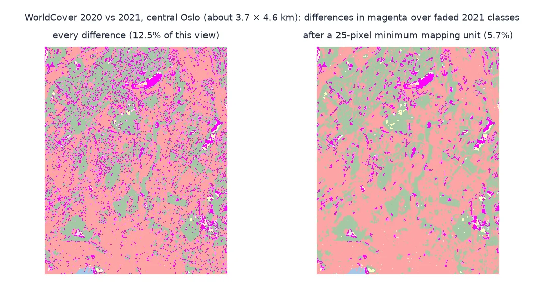
This page differences ESA WorldCover 2020 (v100) and 2021 (v200) for Oslo, measures the patches the differences form, and shows what minimum mapping units of different sizes keep.

Quick answer

Find changed pixels, group them into connected patches, and look at the size distribution before trusting any total:

changed = (Y2020 != Y2021) & INSIDE
labels, n = ndimage.label(changed, structure=np.ones((3, 3)))
sizes = np.bincount(labels.ravel())[1:]
print(f"{changed.sum() / INSIDE.sum():.1%} of Oslo's pixels differ, in {n:,} patches; median patch {np.median(sizes):.0f} pixels")
print(f"patches of 1–4 pixels: {(sizes <= 4).mean():.0%} of patches, {sizes[sizes <= 4].sum() / sizes.sum():.0%} of changed pixels")

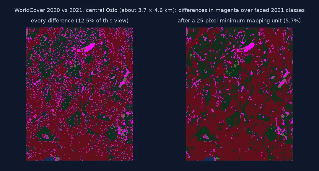
7.6% of Oslo's pixels differ, in 56,776 patches; median patch 4 pixels
patches of 1–4 pixels: 54% of patches, 8% of changed pixels

Patches not pixels, what changed, a minimum mapping unit

1. Look at patches, not pixels

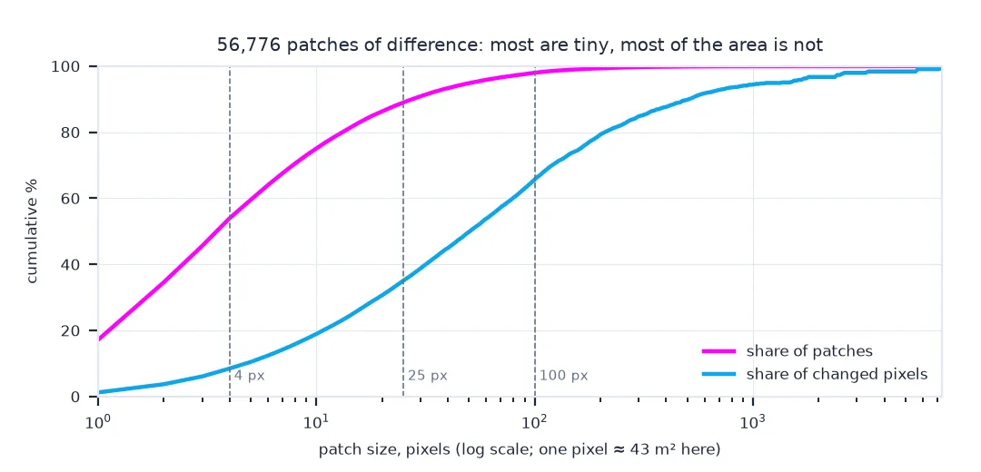
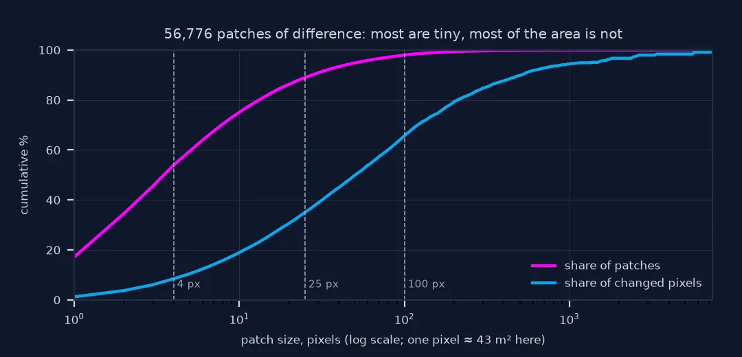
Speckle dominates the number of patches but not necessarily the area. The cumulative share of changed pixels by patch size shows where the change sits:

px_m2 = 43.2                                              # one 1/12,000° pixel at Oslo's latitude
for k in (1, 4, 10, 25, 100, 1000):
    print(f"patches up to {k:>4} pixels (~{k * px_m2 / 1e4:>5.2f} ha): {(sizes <= k).mean():5.1%} of patches, {sizes[sizes <= k].sum() / sizes.sum():5.1%} of changed pixels")

patches up to    1 pixels (~ 0.00 ha): 17.1% of patches,  1.2% of changed pixels
patches up to    4 pixels (~ 0.02 ha): 53.9% of patches,  8.5% of changed pixels
patches up to   10 pixels (~ 0.04 ha): 75.1% of patches, 18.9% of changed pixels
patches up to   25 pixels (~ 0.11 ha): 89.0% of patches, 35.0% of changed pixels
patches up to  100 pixels (~ 0.43 ha): 98.0% of patches, 65.7% of changed pixels
patches up to 1000 pixels (~ 4.32 ha): 100.0% of patches, 94.3% of changed pixels

2. Look at what changed

Rank the transitions. Pairs of classes that are easy to confuse, or edge classes such as trees in gardens, are the first suspects:

pairs = pd.Series(list(zip(Y2020[changed], Y2021[changed]))).value_counts(normalize=True).head(6) * 100
print(pairs.rename(lambda p: f"{WC[p[0]]} → {WC[p[1]]}").round(1).to_string())

Tree cover → Built-up       43.2
Tree cover → Grassland      14.9
Grassland → Tree cover       6.6
Grassland → Cropland         5.8
Cropland → Grassland         5.2
Bare/sparse → Tree cover     3.8

Tree cover to built-up makes up 43% of the differences, which would mean a thirtieth of Oslo built over in a single year. It is far more likely the newer algorithm drawing built-up land differently through the city's tree-lined suburbs. The next three pairs are classic confusions: grassland with trees and with cropland.

3. Apply a minimum mapping unit

rasterio.features.sieve removes patches below a size, replacing them with their surroundings. Apply it to the change mask and see what survives:

for mmu in (4, 25, 100):
    kept = features.sieve(changed.astype(np.uint8), size=mmu, connectivity=8) > 0
    print(f"MMU {mmu:>3} pixels (~{mmu * px_m2 / 1e4:.2f} ha): changed share {kept.sum() / INSIDE.sum():.2%}, "
          f"{ndimage.label(kept, structure=np.ones((3, 3)))[1]:,} patches remain")

MMU   4 pixels (~0.02 ha): changed share 7.17%, 30,896 patches remain
MMU  25 pixels (~0.11 ha): changed share 5.06%, 6,526 patches remain
MMU 100 pixels (~0.43 ha): changed share 2.68%, 1,164 patches remain

A minimum mapping unit of about a tenth of a hectare removes nine in ten patches but only a third of the changed area; at 0.4 ha the changed share falls from 7.6% to 2.7%. What remains is not proven change either, as the largest patches show.

Where the large change patches are

The data used on this page

ESA WorldCover 2020 (v100) and 2021 (v200), 10 m, tiles N57E009 and N60E009 from the public esa-worldcover S3 bucket, read as one window over the municipality of Oslo (boundary from geoBoundaries Norway ADM2, Geonorge, CC BY 4.0). Both versions share the same grid.

from pathlib import Path

import geopandas as gpd
import numpy as np
import pandas as pd
import rasterio
import requests
from rasterio import features
from rasterio.merge import merge
from scipy import ndimage

Path("data").mkdir(exist_ok=True)
BUCKET = "https://esa-worldcover.s3.eu-central-1.amazonaws.com"
F = Path("data/nor_adm2.geojson")
if not F.exists():
    F.write_bytes(requests.get("https://github.com/wmgeolab/geoBoundaries/raw/9469f09/releaseData/gbOpen/NOR/ADM2/geoBoundaries-NOR-ADM2.geojson", timeout=300).content)
adm2 = gpd.read_file(F)
OSLO = adm2[adm2.shapeName.str.startswith("Oslo")]
tiles = ("N57E009", "N60E009")
m20, T = merge([rasterio.open(f"/vsicurl/{BUCKET}/v100/2020/map/ESA_WorldCover_10m_2020_v100_{t}_Map.tif") for t in tiles], bounds=tuple(OSLO.total_bounds))
m21, T21 = merge([rasterio.open(f"/vsicurl/{BUCKET}/v200/2021/map/ESA_WorldCover_10m_2021_v200_{t}_Map.tif") for t in tiles], bounds=tuple(OSLO.total_bounds))
Y2020, Y2021 = m20[0], m21[0]
INSIDE = features.geometry_mask(OSLO.geometry, Y2021.shape, T, invert=True) & (Y2020 > 0) & (Y2021 > 0)
WC = {10: "Tree cover", 20: "Shrubland", 30: "Grassland", 40: "Cropland", 50: "Built-up", 60: "Bare/sparse", 70: "Snow/ice",
      80: "Water", 90: "Herbaceous wetland", 95: "Mangroves", 100: "Moss/lichen"}
print(f"same grid: {T == T21}; {INSIDE.sum():,} pixels inside Oslo")

same grid: True; 10,448,698 pixels inside Oslo

Example 1: where the big patches are

big = np.argsort(sizes)[::-1][:3] + 1
for k in big:
    rows, cols = np.nonzero(labels == k)
    lon, lat = T * (cols.mean(), rows.mean())
    tr = pd.Series(list(zip(Y2020[rows, cols], Y2021[rows, cols]))).value_counts().index[0]
    print(f"patch of {sizes[k - 1]:,} pixels at {lat:.4f} N, {lon:.4f} E: mostly {WC[tr[0]]} → {WC[tr[1]]}")

patch of 7,336 pixels at 59.8947 N, 10.7774 E: mostly Grassland → Cropland
patch of 5,674 pixels at 60.0660 N, 10.5860 E: mostly Grassland → Water
patch of 3,305 pixels at 59.9652 N, 10.6307 E: mostly Grassland → Cropland

Map errors show up as change

Every land cover map has errors, and they concentrate on class edges and between similar classes. When two maps are differenced, each map's errors appear as change, so the change map shows the union of both maps' errors along with any real change. The errors are mostly small and scattered because they follow edges and mixed pixels; real change, such as a new housing estate or a felled stand, usually forms compact patches. That difference in shape is what a minimum mapping unit exploits.

Here the two maps were also made with different versions of the algorithm, so their differences mix method and change; the comparison is a useful worst case. Product series designed for change, such as NLCD or Annual NLCD, detect change first and relabel only the changed pixels, which suppresses much of this. Whatever the source, report change with its minimum mapping unit, and look at the largest patches by eye before trusting a total.

Connectivity, sieving and majority filters

• Connectivity: 8-connectivity joins diagonal neighbours into one patch; 4-connectivity splits them. State which.
• Pixel area varies: in EPSG:4326 an MMU in pixels is a different area at each latitude; set it in hectares and convert.
• Sieve the maps or the change? Sieving each map before differencing removes isolated pixels from both; sieving the change mask removes small changes. They give different results.
• Majority filters (scipy.ndimage with a mode filter) smooth class maps but also erode thin real features such as rivers and roads.
• Accuracy: an MMU removes noise but not systematic disagreement; large patches can still be method differences.

Internal links

• How to read ESA WorldCover tiles — the data
• How to build a land cover change matrix — change from a series built for it

FAQ

Why does my land cover change map look noisy?

Each map's classification errors, concentrated on edges and between similar classes, appear as change when the maps are differenced.

What is a minimum mapping unit?

The smallest patch a map treats as a feature; change patches smaller than it are dropped or merged into their surroundings.

How do I remove small patches from a raster in Python?

rasterio.features.sieve(array, size=n) replaces connected patches smaller than n pixels with the value of their largest neighbour.

Can I compare ESA WorldCover 2020 and 2021 for change?

Not reliably: the two versions were made with different algorithms, so their differences mix method changes with real change.