Why Are My Land Cover Areas Wrong in Degrees?

Problem statement

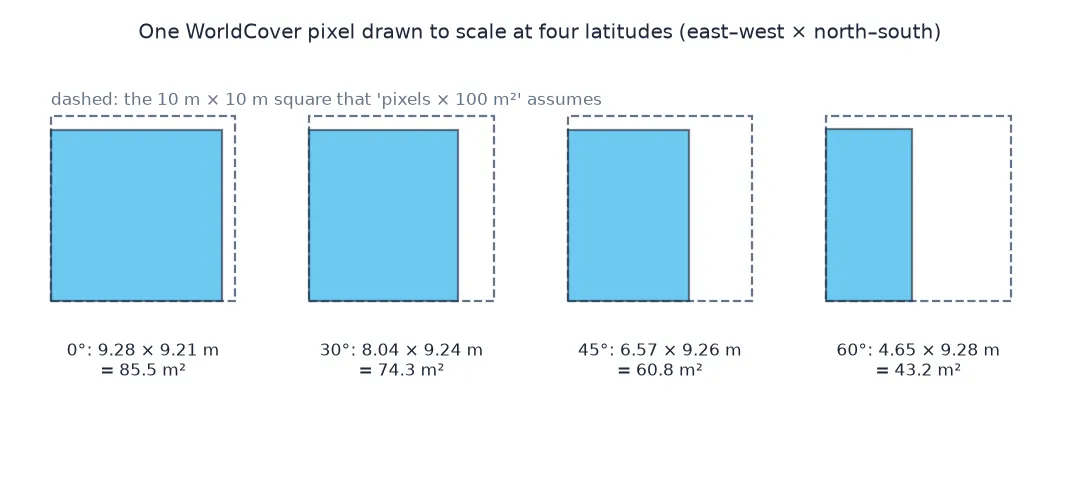
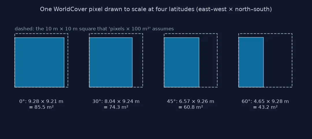
ESA WorldCover is "10 m land cover", so the area of a class must be its pixel count times 100 m². For Oslo that gives the municipality an area of 1,045 km². Its boundary encloses 452 km². The map is not in metres: WorldCover pixels are 1/12,000 of a degree in each direction, which is about 9.3 m north–south everywhere, but east–west shrinks with the cosine of latitude. At Oslo's 60° N a pixel covers about 43 m², not 100.

The same trap applies to any land cover or raster product in a geographic CRS (EPSG:4326): Dynamic World exports, many global forest and water products, climate grids. This page measures the error for Oslo and shows two correct ways to compute class areas.

Quick answer

Give every pixel row its true area on the ellipsoid, then sum by class:

lat_top = TRANSFORM.f + np.arange(WC.shape[0]) * TRANSFORM.e          # latitude of each row's top edge
res = TRANSFORM.a
row_m2 = np.array([abs(GEOD.polygon_area_perimeter([0, res, res, 0], [la, la, la - res, la - res])[0]) for la in lat_top])
pix_m2 = np.broadcast_to(row_m2[:, None], WC.shape)
naive = (WC > 0).sum() * 100 / 1e6
true = pix_m2[WC > 0].sum() / 1e6
print(f"Oslo: {naive:,.0f} km² as count × 100 m², {true:,.0f} km² with true pixel areas ({naive / true:.2f}x too large)")
print(f"a pixel here covers {row_m2.min():.1f}–{row_m2.max():.1f} m²")

Oslo: 1,045 km² as count × 100 m², 451 km² with true pixel areas (2.32x too large)
a pixel here covers 43.0–43.4 m²

Check CRS and pixel size, see the latitude effect, reproject

1. Check the CRS and the pixel size

with rasterio.open("data/oslo_worldcover.tif") as src:
    print(src.crs, f"pixel {src.res[0]:.10f}° x {src.res[1]:.10f}°")
lat = 60.0
ns = GEOD.inv(10, lat, 10, lat + res)[2]; ew = GEOD.inv(10, lat, 10 + res, lat)[2]
print(f"at {lat}° N one pixel is {ns:.2f} m north–south and {ew:.2f} m east–west")

EPSG:4326 pixel 0.0000833333° x 0.0000833333°
at 60.0° N one pixel is 9.28 m north–south and 4.65 m east–west

2. See how the error grows with latitude

for la in (0, 30, 45, 60, 70):
    a = abs(GEOD.polygon_area_perimeter([0, res, res, 0], [la, la, la + res, la + res])[0])
    print(f"{la:2d}°: true pixel area {a:6.1f} m²; count × 100 m² overstates by {100 / a:.2f}x")

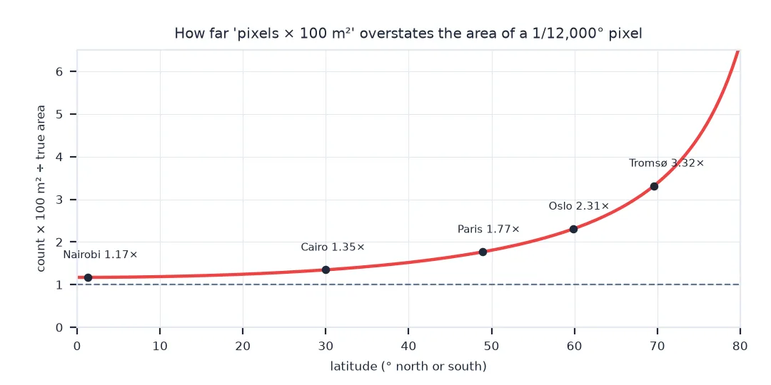
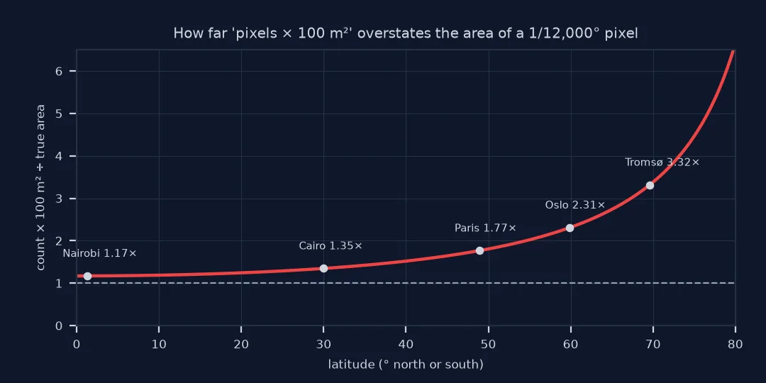
 0°: true pixel area   85.5 m²; count × 100 m² overstates by 1.17x
30°: true pixel area   74.3 m²; count × 100 m² overstates by 1.35x
45°: true pixel area   60.8 m²; count × 100 m² overstates by 1.64x
60°: true pixel area   43.2 m²; count × 100 m² overstates by 2.32x
70°: true pixel area   29.6 m²; count × 100 m² overstates by 3.38x

Even at the equator the pixel is about 85 m², not 100, because 1/12,000 of a degree is 9.3 m, not 10.

3. Or reproject to an equal-area CRS, with nearest neighbour

Reprojecting to a metric CRS gives pixels of known size. It must use nearest-neighbour resampling, so no new class values appear:

dst_t, w, h = calculate_default_transform("EPSG:4326", "EPSG:25833", WC.shape[1], WC.shape[0], *array_bounds(*WC.shape, TRANSFORM), resolution=10)
utm = np.zeros((h, w), np.uint8)
reproject(WC, utm, src_transform=TRANSFORM, src_crs="EPSG:4326", dst_transform=dst_t, dst_crs="EPSG:25833", resampling=Resampling.nearest)
print(f"UTM 33N, 10 m pixels: {(utm > 0).sum() * 100 / 1e6:,.0f} km²; new values created: {sorted(set(np.unique(utm)) - set(np.unique(WC)))}")

UTM 33N, 10 m pixels: 452 km²; new values created: []

UTM zone 33 is not strictly equal-area, but within a zone its area distortion is a fraction of a per cent, well below the classification's own error.

Class areas, and why shares survive

The data used on this page

ESA WorldCover 2021 v200 (tiles N57E009 and N60E009 from the public esa-worldcover S3 bucket) and the municipality of Oslo from geoBoundaries Norway ADM2 (Geonorge, CC BY 4.0). Pixel areas are computed on the WGS 84 ellipsoid with pyproj.Geod.

from pathlib import Path

import geopandas as gpd
import numpy as np
import pandas as pd
import rasterio
import rasterio.mask
import requests
from pyproj import Geod
from rasterio.merge import merge
from rasterio.transform import array_bounds
from rasterio.warp import Resampling, calculate_default_transform, reproject

Path("data").mkdir(exist_ok=True)
BUCKET = "https://esa-worldcover.s3.eu-central-1.amazonaws.com"
F = Path("data/nor_adm2.geojson")
if not F.exists():
    F.write_bytes(requests.get("https://github.com/wmgeolab/geoBoundaries/raw/9469f09/releaseData/gbOpen/NOR/ADM2/geoBoundaries-NOR-ADM2.geojson", timeout=300).content)
adm2 = gpd.read_file(F)
OSLO = adm2[adm2.shapeName.str.startswith("Oslo")]
if not Path("data/oslo_worldcover.tif").exists():
    srcs = [rasterio.open(f"/vsicurl/{BUCKET}/v200/2021/map/ESA_WorldCover_10m_2021_v200_{n}_Map.tif") for n in ("N57E009", "N60E009")]
    mosaic, tr = merge(srcs, bounds=tuple(OSLO.total_bounds))
    with rasterio.open("data/oslo_worldcover.tif", "w", driver="GTiff", height=mosaic.shape[1], width=mosaic.shape[2], count=1,
                       dtype="uint8", crs="EPSG:4326", transform=tr, nodata=0, compress="deflate") as dst:
        dst.write(mosaic)
with rasterio.open("data/oslo_worldcover.tif") as src:
    wc, TRANSFORM = rasterio.mask.mask(src, OSLO.geometry, crop=True, nodata=0)
WC = wc[0]
GEOD = Geod(ellps="WGS84")
WC_CLASSES = {10: "Tree cover", 20: "Shrubland", 30: "Grassland", 40: "Cropland", 50: "Built-up", 60: "Bare/sparse vegetation",
              70: "Snow and ice", 80: "Permanent water bodies", 90: "Herbaceous wetland", 95: "Mangroves", 100: "Moss and lichen"}
print(f"Oslo boundary: {OSLO.to_crs(25833).area.sum() / 1e6:,.0f} km² in UTM 33N; WorldCover window {WC.shape[1]} x {WC.shape[0]} pixels")

Oslo boundary: 452 km² in UTM 33N; WorldCover window 5547 x 3910 pixels

Example 1: class areas, and why shares survive

classes = sorted(set(np.unique(WC)) - {0})
t = pd.DataFrame({"naive km²": [(WC == c).sum() * 100 / 1e6 for c in classes],
                  "true km²": [pix_m2[WC == c].sum() / 1e6 for c in classes]}, index=[WC_CLASSES[c] for c in classes])
t["share (count)"] = t["naive km²"] / t["naive km²"].sum() * 100
t["share (area)"] = t["true km²"] / t["true km²"].sum() * 100
print(t.round(1).sort_values("true km²", ascending=False).to_string())

                        naive km²  true km²  share (count)  share (area)
Tree cover                  781.3     337.4           74.8          74.8
Built-up                    144.0      62.3           13.8          13.8
Permanent water bodies       59.6      25.7            5.7           5.7
Grassland                    42.3      18.3            4.0           4.0
Cropland                     15.8       6.8            1.5           1.5
Bare/sparse vegetation        1.2       0.5            0.1           0.1
Herbaceous wetland            0.7       0.3            0.1           0.1

Within one city, pixel areas barely vary, so class shares come out the same either way. Areas in km² do not, and shares do not either over a region spanning many degrees of latitude.

Angular units, uneven distances

A geographic CRS has angular units. A pixel of a fixed angle covers a fixed distance north–south (a degree of latitude is about 111 km everywhere) but an east–west distance proportional to the cosine of latitude. "10 m" in a product's name describes its resolution near the equator, roughly; it is not a pixel area. Counting pixels and multiplying by a nominal area is only right in a projected, equal-area CRS.

The correction is cheap because pixel area depends only on the row. One ellipsoidal area per row, broadcast across the columns, weights every pixel exactly; this is the approach used for global land cover statistics. Reprojecting is the alternative when the data are needed in metres anyway, provided the resampling is nearest neighbour and the CRS is suitable for the region.

Sphere versus ellipsoid and global sums

• Sphere vs ellipsoid: the spherical formula R² Δλ (sin φ₁ − sin φ₂) is a close approximation; pyproj.Geod gives the ellipsoidal area at little extra cost.
• Equator: even there a pixel is about 9.2 m north–south by 9.3 m east–west, 85.5 m², so count × 100 m² overstates by 17%.
• Other "10 m" products: Sentinel-2 bands in their UTM CRS really are 10 m pixels; only products delivered in EPSG:4326 need the correction.
• Masks: the boundary mask keeps whole pixels by their centre; that error is tiny next to the latitude error.
• Global sums: summing pixel counts across latitudes mixes pixel sizes from 85 m² to almost nothing near the poles.

Internal links

• How to read ESA WorldCover tiles — the data
• Why is my wildfire area too large? — the same kind of error with Web Mercator

FAQ

Why is the area of my WorldCover class too large?

WorldCover pixels are 1/12,000 of a degree, not 10 m squares. Away from the equator they cover much less than 100 m²: about 43 m² at 60° N.

How do I calculate land cover area from a raster in EPSG:4326?

Compute the true area of one pixel per row with pyproj.Geod, multiply each pixel by its row's area, and sum by class; or reproject to an equal-area CRS with nearest-neighbour resampling.

Are class percentages wrong too?

Within a small area, hardly: all pixels have nearly the same area. Over many degrees of latitude, yes.

What is the pixel size of ESA WorldCover?

1/12,000 of a degree (0.0000833°), about 9.3 m north–south and 9.3 m × cos(latitude) east–west.