
How to Summarise Land Cover by Polygon in Python
On this page
Problem statement
"What does each city in the county look like?" asks for land cover composition by polygon: the share of each class inside each boundary. It looks like a job for a zonal statistics function, and most of them default to mean, min, max and sum. On a categorical raster those numbers are nonsense: the mean of class codes 21 and 82 is 51.5, which is not a land cover at all. What a categorical raster needs is a count of pixels per class per zone, turned into areas and shares.
This page summarises NLCD 2021 by city for the incorporated places of Williamson County, Texas, and compares their composition with 2001.
Quick answer
Rasterise the polygons onto the land cover grid, then cross-tabulate zone against class:
zones = features.rasterize([(g, k + 1) for k, g in enumerate(PLACES.geometry)], out_shape=LC[2021].shape, transform=TRANSFORM)
inside = zones > 0
counts = pd.crosstab(pd.Series(zones[inside], name="zone"), pd.Series(LC[2021][inside], name="class"))
counts.index = PLACES.NAME.iloc[counts.index - 1]
shares = counts.T.groupby(GROUP).sum().T.pipe(lambda t: t.div(t.sum(axis=1), axis=0) * 100)
print(shares.round(0).astype(int).sort_values("Developed", ascending=False).to_string())
class Agriculture Barren Developed Forest Grassland Shrub Water Wetland
NAME
Granger 10 0 88 0 2 0 0 0
Thrall 20 0 74 0 3 2 0 0
Round Rock 2 0 73 5 16 0 1 2
Cedar Park 0 1 73 16 6 3 1 0
Bartlett 15 0 71 0 13 0 0 0
Florence 4 0 56 5 27 6 0 1
Hutto 31 1 52 0 13 2 0 2
Jarrell 2 1 52 1 44 0 0 0
Liberty Hill 0 2 49 11 29 10 0 0
Leander 0 1 49 27 16 7 0 1
Georgetown 2 1 44 18 27 2 3 2
Taylor 47 0 34 1 11 3 0 4
Coupland 66 0 23 0 4 5 1 1
Weir 15 1 21 2 57 0 1 4
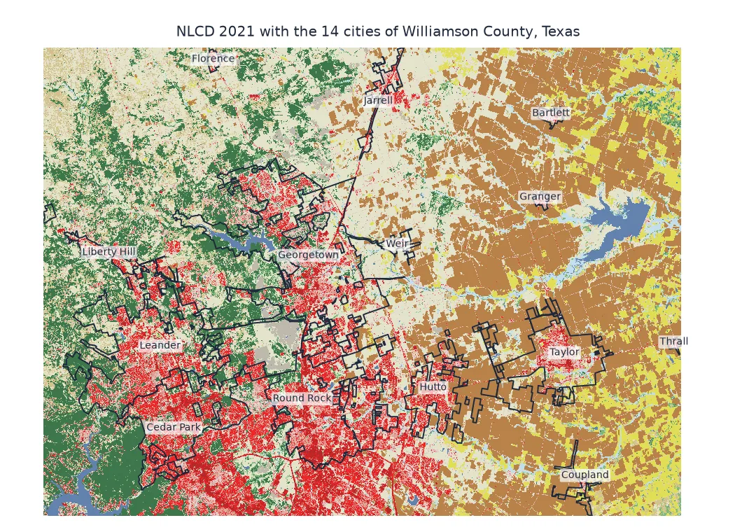
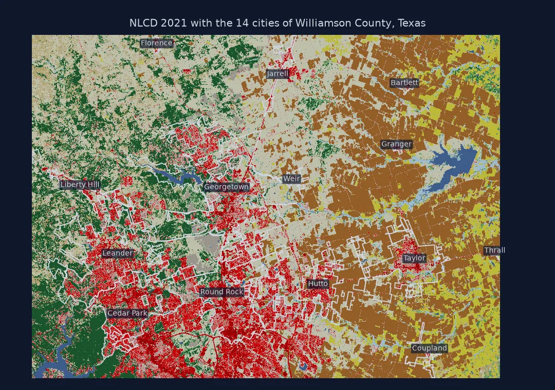
Why the mean is wrong, areas and shares, same zones over time
1. See why the mean is wrong
A zonal mean of the class codes runs without complaint and produces numbers between codes:
codes_mean = pd.Series({PLACES.NAME.iloc[k - 1]: LC[2021][zones == k].mean() for k in range(1, len(PLACES) + 1)})
print(codes_mean.round(1).sort_values().head(4).to_string())
print("those 'classes' do not exist: NLCD codes are", sorted(NLCD_CLASSES))
Granger 29.0
Cedar Park 29.8
Round Rock 34.3
Thrall 36.4
those 'classes' do not exist: NLCD codes are [11, 12, 21, 22, 23, 24, 31, 41, 42, 43, 52, 71, 81, 82, 90, 95]
A city with a mean code of about 30 is not close to class 31, barren land; it is a mix of developed (21–24) and cropland or grass (71–82). Only counts per class mean anything.
2. Report areas as well as shares
Shares hide size. Convert counts to square kilometres:
km2 = counts.T.groupby(GROUP).sum().T * PIXEL_KM2
print(km2[["Developed", "Grassland", "Agriculture", "Forest"]].round(1).sort_values("Developed", ascending=False).head(6).to_string())
class Developed Grassland Agriculture Forest
NAME
Round Rock 72.9 15.7 2.3 4.8
Georgetown 69.3 42.6 3.8 28.5
Leander 49.1 15.9 0.2 27.0
Cedar Park 48.6 4.3 0.0 10.7
Taylor 19.9 6.2 27.7 0.7
Hutto 18.7 4.6 11.2 0.1
3. Compare years with the same zones
Reuse the same zone raster for 2001 so every difference is a change in land cover, not in the polygons:
dev = {y: pd.Series(np.bincount(zones[inside], weights=np.isin(LC[y][inside], [21, 22, 23, 24]), minlength=len(PLACES) + 1)[1:] * PIXEL_KM2,
                    index=PLACES.NAME) for y in (2001, 2021)}
change = pd.DataFrame({"2001 km²": dev[2001], "2021 km²": dev[2021]})
change["growth"] = change["2021 km²"] / change["2001 km²"] - 1
print(change.sort_values("2021 km²", ascending=False).head(6).round(2).to_string(formatters={"growth": "{:+.0%}".format}))
2001 km² 2021 km² growth
NAME
Round Rock 50.89 72.90 +43%
Georgetown 39.37 69.31 +76%
Leander 18.08 49.12 +172%
Cedar Park 26.52 48.57 +83%
Taylor 17.05 19.85 +16%
Hutto 4.22 18.75 +344%
Hutto's developed area more than quadrupled and Leander's nearly tripled, while Taylor, among the farmland of the east, grew by 16%.
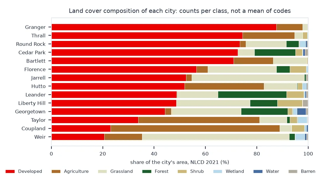
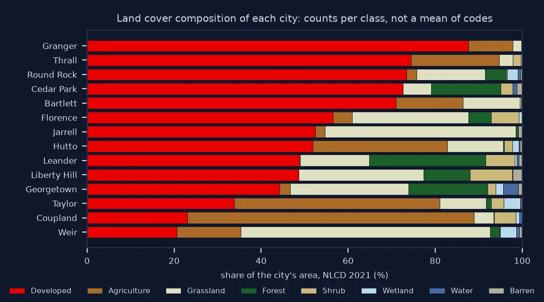
The most and least developed city
The data used on this page
NLCD 2001 and 2021 (2021 release, 30 m) for Williamson County, Texas, from MRLC's WCS, and the 2023 Census cartographic boundary file of Texas places, keeping incorporated places whose interior point lies in the county; each is summarised whole, including any part in a neighbouring county. Place boundaries are 2023 boundaries for both years.
import time
from pathlib import Path

import geopandas as gpd
import numpy as np
import pandas as pd
import rasterio
import requests
from rasterio import features

Path("data").mkdir(exist_ok=True)
WCS = "https://www.mrlc.gov/geoserver/mrlc_download/wcs"
for name, url in {"cb_2023_us_county_20m.zip": "https://www2.census.gov/geo/tiger/GENZ2023/shp/cb_2023_us_county_20m.zip",
                  "cb_2023_48_place_500k.zip": "https://www2.census.gov/geo/tiger/GENZ2023/shp/cb_2023_48_place_500k.zip"}.items():
    if not Path("data", name).exists():
        Path("data", name).write_bytes(requests.get(url, timeout=300).content)
COUNTY = gpd.read_file("data/cb_2023_us_county_20m.zip").query("GEOID == '48491'").to_crs(5070)
places = gpd.read_file("data/cb_2023_48_place_500k.zip").to_crs(5070)
PLACES = places[(places.LSAD == "25") & places.representative_point().within(COUNTY.union_all())].sort_values("NAME").reset_index(drop=True)
x0, y0, x1, y1 = PLACES.total_bounds
LC = {}
for year in (2001, 2021):
    path = Path(f"data/nlcd_places_{year}.tif")
    if not path.exists():
        for attempt in range(4):
            r = requests.get(WCS, params={"service": "WCS", "version": "2.0.1", "request": "GetCoverage",
                                          "coverageId": f"mrlc_download__NLCD_{year}_Land_Cover_L48",
                                          "subset": [f"X({x0},{x1})", f"Y({y0},{y1})"], "format": "image/geotiff"}, timeout=300)
            if r.status_code < 500:
                break
            time.sleep(15 * (attempt + 1))
        r.raise_for_status()
        path.write_bytes(r.content)
    with rasterio.open(path) as src:
        LC[year], TRANSFORM = src.read(1), src.transform
PIXEL_KM2 = 30 * 30 / 1e6
NLCD_CLASSES = [11, 12, 21, 22, 23, 24, 31, 41, 42, 43, 52, 71, 81, 82, 90, 95]
GROUP = {11: "Water", 21: "Developed", 22: "Developed", 23: "Developed", 24: "Developed", 31: "Barren", 41: "Forest", 42: "Forest",
         43: "Forest", 52: "Shrub", 71: "Grassland", 81: "Agriculture", 82: "Agriculture", 90: "Wetland", 95: "Wetland"}
print(f"{len(PLACES)} cities: {', '.join(PLACES.NAME)}")
14 cities: Bartlett, Cedar Park, Coupland, Florence, Georgetown, Granger, Hutto, Jarrell, Leander, Liberty Hill, Round Rock, Taylor, Thrall, Weir
Example 1: the most and least developed city
dev_share = shares["Developed"].sort_values()
print(f"least developed: {dev_share.index[0]} {dev_share.iloc[0]:.0f}%; most developed: {dev_share.index[-1]} {dev_share.iloc[-1]:.0f}%")
agri = shares["Agriculture"].idxmax()
print(f"most agricultural: {agri}, {shares.loc[agri, 'Agriculture']:.0f}% agriculture and {shares.loc[agri, 'Developed']:.0f}% developed")
least developed: Weir 21%; most developed: Granger 88%
most agricultural: Coupland, 66% agriculture and 23% developed
Zonal statistics on classes is a cross-tabulation
Zonal statistics on a categorical raster is a cross-tabulation: each pixel contributes its zone and its class, and the result is a count for every pair. Shares follow by dividing each zone's row by its total, areas by multiplying by the pixel area. The same table gives a majority class (the largest count) or a diversity index if needed. What it never gives is an average class, because class codes are labels, not quantities.
Rasterising polygons assigns each pixel wholly to the zone containing its centre, which is exact enough for cities of tens of square kilometres at 30 m. For small or thin polygons, tools that weight partial pixels by their covered fraction (exactextract, or rasterstats with all_touched handled carefully) do better. Whatever the method, the same zone raster must be reused across years, or boundary differences show up as land cover change.
Overlapping polygons, nodata and equal-area CRSs
rasterstats: usecategorical=Truefor counts per class instead of the default statistics.- Overlapping polygons: rasterising gives each pixel to one polygon (the last drawn); overlapping zones need one pass per polygon.
- Nodata: NLCD land cover uses 0 outside the mapped area; drop it before computing shares.
- Boundaries change: cities annex land; with 2023 boundaries, part of a city's "growth" is land that was outside it in 2001.
- Equal-area CRS: count × 900 m² is valid because NLCD is in CONUS Albers.
Internal links
- How to calculate zonal statistics in Python — continuous rasters
- How to build a land cover change matrix — change for the whole county
FAQ
How do I calculate land cover percentages by polygon in Python?
Rasterise the polygons to the land cover grid, cross-tabulate zone against class with pd.crosstab, and divide each row by its total.
Why is the zonal mean of a land cover raster meaningless?
Class codes are labels. Averaging them gives values between codes that correspond to no class.
What is the majority class of a zone?
The class with the largest pixel count in that zone, the idxmax of its row in the cross-tabulation.
Can I use rasterstats for land cover?
Yes, with categorical=True, which returns the count of each class in each polygon.