Why Are the Colours on My Land Cover Map Wrong?

On this page

Problem statement

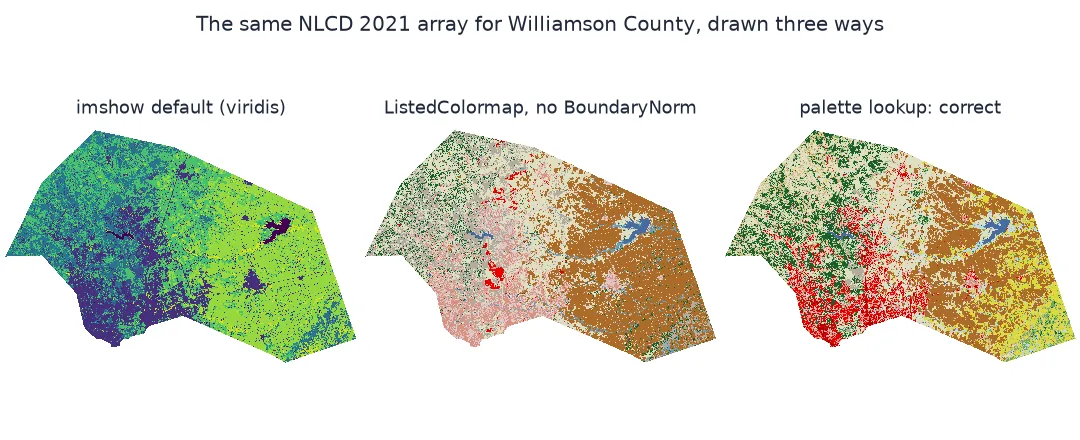
You plot a land cover raster with plt.imshow and the map is a smear of yellows and purples in which forest and grassland look alike. You give it the official NLCD colours as a ListedColormap, and now evergreen forest is grey and pasture looks like crops. Nothing is wrong with the data. imshow treats the class codes as a continuous quantity and stretches them across the colormap, so a colour is chosen by where a code falls between the smallest and largest code, not by which class it is.

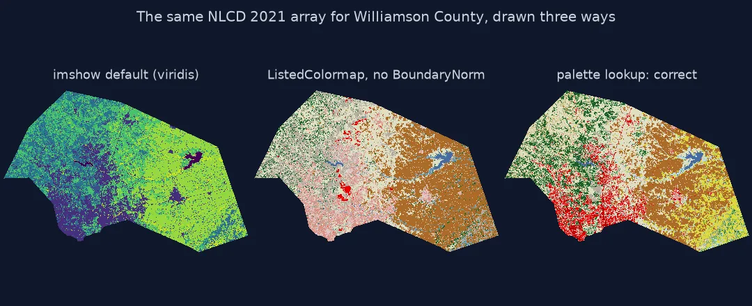
This page draws NLCD 2021 for Williamson County, Texas, three ways and measures which classes get the wrong colour in each, then shows two ways to get the official colours exactly.

Quick answer

Map each code to its colour directly with a lookup array, and draw RGB:

PALETTE = np.zeros((256, 3))
for code, hexcol in NLCD_COLORS.items():
    PALETTE[code] = matplotlib.colors.to_rgb(hexcol)
rgb = PALETTE[LC]                                  # (rows, cols, 3); code 0 stays black, set it to the background
rgb[LC == 0] = 1.0
fig, ax = plt.subplots(figsize=(6, 4))
ax.imshow(rgb, interpolation="nearest"); ax.set_axis_off()
fig.savefig("data/williamson_nlcd.png", dpi=150)
print(f"{len(np.unique(LC[LC > 0]))} classes drawn, each in its own colour; image {rgb.shape[1]} x {rgb.shape[0]}")

15 classes drawn, each in its own colour; image 2845 x 1884

Three renderings of the same land cover array: with matplotlib's default viridis colormap the classes become shades of purple, green and yellow with no meaning; with a list of the official colours but no BoundaryNorm, forests turn grey and pink and developed land turns pale; with a palette lookup the map shows the official NLCD colours, red towns, green forest and brown crops. — The data are the same in all three. Only the third maps codes to colours.

Continuous colormaps, unnormed lists, a boundary norm

1. See what a continuous colormap does

With the default colormap, colour depends on the code's position between 11 and 95. Codes close together get nearly the same colour:

norm = Normalize(min(CODES), max(CODES))
v = np.array([matplotlib.colormaps["viridis"](norm(c))[:3] for c in CODES]) * 255
d = np.sqrt(((v[:, None] - v[None]) ** 2).sum(-1))
close = [(CODES[i], CODES[j]) for i, j in zip(*np.triu_indices(len(CODES), 1)) if d[i, j] < 20]
print(f"{len(close)} pairs of classes drawn in nearly the same colour (RGB distance under 20), e.g. {close[:4]}")

10 pairs of classes drawn in nearly the same colour (RGB distance under 20), e.g. [(21, 22), (21, 23), (21, 24), (22, 23)]

2. See what a ListedColormap without a norm does

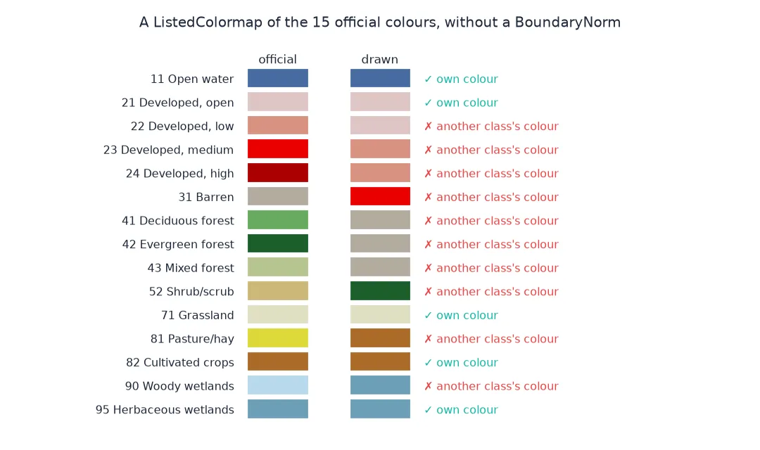
A ListedColormap with one colour per class is still indexed by the stretched value, so codes land on their neighbours' colours:

cmap = ListedColormap([NLCD_COLORS[c] for c in CODES])
drawn = {c: CODES[[np.allclose(cmap(norm(c)), matplotlib.colors.to_rgba(NLCD_COLORS[k])) for k in CODES].index(True)] for c in CODES}
wrong = {c: k for c, k in drawn.items() if c != k}
print(f"{len(wrong)} of {len(CODES)} classes drawn in another class's colour:")
print({f"{c} {NAMES[c]}": f"{k} {NAMES[k]}" for c, k in list(wrong.items())[:5]})

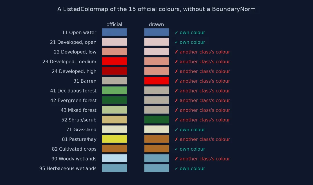
10 of 15 classes drawn in another class's colour:
{'22 Developed, low': '21 Developed, open', '23 Developed, medium': '22 Developed, low', '24 Developed, high': '22 Developed, low', '31 Barren': '23 Developed, medium', '41 Deciduous forest': '31 Barren'}

Swatches comparing official and drawn colours for 15 NLCD classes under a ListedColormap without a BoundaryNorm: open water, developed open space, grassland, cultivated crops and herbaceous wetlands get their own colours; the other 10 get another class's colour, for example evergreen forest drawn in barren grey and pasture in crop brown. — Ten of fifteen classes take a neighbour's colour.

3. Or use a BoundaryNorm

If a colormap is needed (for a colorbar-style legend or a library that wants one), give it boundaries between the codes so each code falls in its own bin:

bounds = [c - 0.5 for c in CODES] + [CODES[-1] + 0.5]
bnorm = BoundaryNorm(bounds, cmap.N)
ok = all(np.allclose(cmap(bnorm(c)), matplotlib.colors.to_rgba(NLCD_COLORS[c])) for c in CODES)
print(f"with BoundaryNorm, every class gets its own colour: {ok}")

with BoundaryNorm, every class gets its own colour: True

A legend for the classes present

The data used on this page

NLCD 2021 (30 m) for Williamson County, Texas, from MRLC's WCS, masked to the 2023 Census county outline. Colours are NLCD's official legend colours, which the WCS files also carry as an embedded palette.

import time
from pathlib import Path

import geopandas as gpd
import matplotlib
matplotlib.use("Agg")
import matplotlib.pyplot as plt
import numpy as np
import rasterio
import rasterio.mask
import requests
from matplotlib.colors import BoundaryNorm, ListedColormap, Normalize

Path("data").mkdir(exist_ok=True)
if not Path("data/cb_2023_us_county_20m.zip").exists():
    Path("data/cb_2023_us_county_20m.zip").write_bytes(requests.get("https://www2.census.gov/geo/tiger/GENZ2023/shp/cb_2023_us_county_20m.zip", timeout=300).content)
COUNTY = gpd.read_file("data/cb_2023_us_county_20m.zip").query("GEOID == '48491'").to_crs(5070)
path = Path("data/nlcd_2021.tif")
if not path.exists():
    x0, y0, x1, y1 = COUNTY.total_bounds
    for attempt in range(4):
        r = requests.get("https://www.mrlc.gov/geoserver/mrlc_download/wcs", params={"service": "WCS", "version": "2.0.1", "request": "GetCoverage",
                         "coverageId": "mrlc_download__NLCD_2021_Land_Cover_L48", "subset": [f"X({x0},{x1})", f"Y({y0},{y1})"], "format": "image/geotiff"}, timeout=300)
        if r.status_code < 500:
            break
        time.sleep(15 * (attempt + 1))
    r.raise_for_status()
    path.write_bytes(r.content)
with rasterio.open(path) as src:
    LC = rasterio.mask.mask(src, COUNTY.geometry, crop=True, nodata=0)[0][0]
    FILE_PALETTE = src.colormap(1)
NLCD_COLORS = {11: "#466b9f", 21: "#dec5c5", 22: "#d99282", 23: "#eb0000", 24: "#ab0000", 31: "#b3ac9f", 41: "#68ab5f", 42: "#1c5f2c",
               43: "#b5c58f", 52: "#ccb879", 71: "#dfdfc2", 81: "#dcd939", 82: "#ab6c28", 90: "#b8d9eb", 95: "#6c9fb8"}
NAMES = {11: "Open water", 21: "Developed, open", 22: "Developed, low", 23: "Developed, medium", 24: "Developed, high", 31: "Barren",
         41: "Deciduous forest", 42: "Evergreen forest", 43: "Mixed forest", 52: "Shrub/scrub", 71: "Grassland", 81: "Pasture/hay",
         82: "Cultivated crops", 90: "Woody wetlands", 95: "Herbaceous wetlands"}
CODES = sorted(NLCD_COLORS)
print(f"{len(CODES)} classes; the file's own palette for 42: {FILE_PALETTE[42]}, official {NLCD_COLORS[42]}")

15 classes; the file's own palette for 42: (28, 95, 44, 255), official #1c5f2c

Example 1: a legend for the classes that are present

present = [c for c in CODES if (LC == c).any()]
handles = [matplotlib.patches.Patch(color=NLCD_COLORS[c], label=f"{NAMES[c]} ({(LC == c).sum() * 900 / 1e6:,.0f} km²)") for c in present]
fig, ax = plt.subplots(figsize=(8, 4))
ax.imshow(rgb, interpolation="nearest"); ax.set_axis_off()
fig.legend(handles=handles, loc="center right", fontsize=7, frameon=False)
fig.savefig("data/williamson_nlcd_legend.png", dpi=150, bbox_inches="tight")
top = max(present, key=lambda c: (LC == c).sum())
print(f"legend with {len(handles)} entries; largest class: {NAMES[top]}, {(LC == top).sum() * 900 / 1e6:,.0f} km²")

legend with 15 entries; largest class: Grassland, 758 km²

Image functions built for continuous data

Matplotlib's image functions are built for continuous data: a norm maps each value to a number between 0 and 1, and the colormap turns that number into a colour. Class codes pass through the same machinery unless told otherwise. The linear norm stretches 11 to 95 across the colormap. A list of 15 colours divides that range into 15 equal slices, and the codes do not sit one per slice: four developed classes in the 20s share the slices around them, the forest classes in the 40s share theirs, and only some codes land where their own colour is.

Four ways to colour class codes.

The fix is to stop treating codes as quantities. A 256-entry palette array indexed by the code is exact and needs no norm at all; it is also how the GeoTIFF's own colour table works. When a colormap is required, a BoundaryNorm with a bin edge halfway between every pair of codes does the same job. Either way, the legend should list classes with their colours, not show a colorbar, which implies an order and a scale that land cover does not have.

Interpolation, file palettes and code zero

Colour problems and fixes.

interpolation="nearest": the default antialiasing can blend neighbouring class colours when an image is drawn smaller than its pixels.
The file's palette: src.colormap(1) returns the GeoTIFF's colour table; it matches the official colours here and can build the palette array directly.
Code 0: give nodata the background colour, or it draws in whatever the palette has at 0 (black here).
Colour blindness: official palettes are not designed for it; red developed against green forest is hard for some readers. Add patterns or labels where it matters.
Rasterio's show: rasterio.plot.show also uses a continuous colormap by default.

Internal links

How to read ESA WorldCover tiles — another product, another official palette
How to reclassify a land cover raster — new classes need a new palette

FAQ

Why are my land cover colours wrong in matplotlib?

imshow stretches class codes across the colormap like continuous values. Map codes to colours with a lookup array, or use a ListedColormap with a BoundaryNorm.

How do I use the official NLCD colours in Python?

Build a 256-row palette array from the official colours (or from the GeoTIFF's colour table) and index it with the raster to get RGB.

Why does a ListedColormap not fix it?

Without a BoundaryNorm, the colours are still assigned by each code's position in the stretched range, not by the code itself.

Should a land cover map have a colorbar?

No. Use a legend listing each class and its colour; a colorbar implies an ordered scale.