Why Are My Land Cover Percentages Wrong?

Problem statement

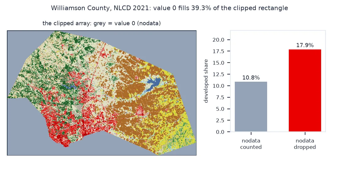
You clip a land cover raster to a county, count the classes, and the percentages come out too small, or one of the "classes" is 0, the biggest of them all. Clipping to a polygon keeps the polygon's bounding box and fills everything outside the polygon with the nodata value, usually 0. Count every value in the array and the outside of the polygon becomes a class, inflating the denominator. Near a coast a rectangle also picks up ocean, part of it mapped as water and part not mapped at all. And a second choice hides inside every percentage: is the share of the total area, or of the land?

This page measures each effect on NLCD 2021: the developed share of Williamson County, Texas, and the land cover of coastal Monterey County, California.

Quick answer

Drop the nodata value before counting, and say which denominator you used:

def shares(arr, drop=(0,)):
    v, n = np.unique(arr, return_counts=True)
    s = pd.Series(n, index=v).drop(list(drop), errors="ignore")
    return s / s.sum() * 100

dev = [21, 22, 23, 24]
print(f"Williamson developed share, nodata counted: {shares(WILL, drop=())[dev].sum():.1f}%; nodata dropped: {shares(WILL)[dev].sum():.1f}%")

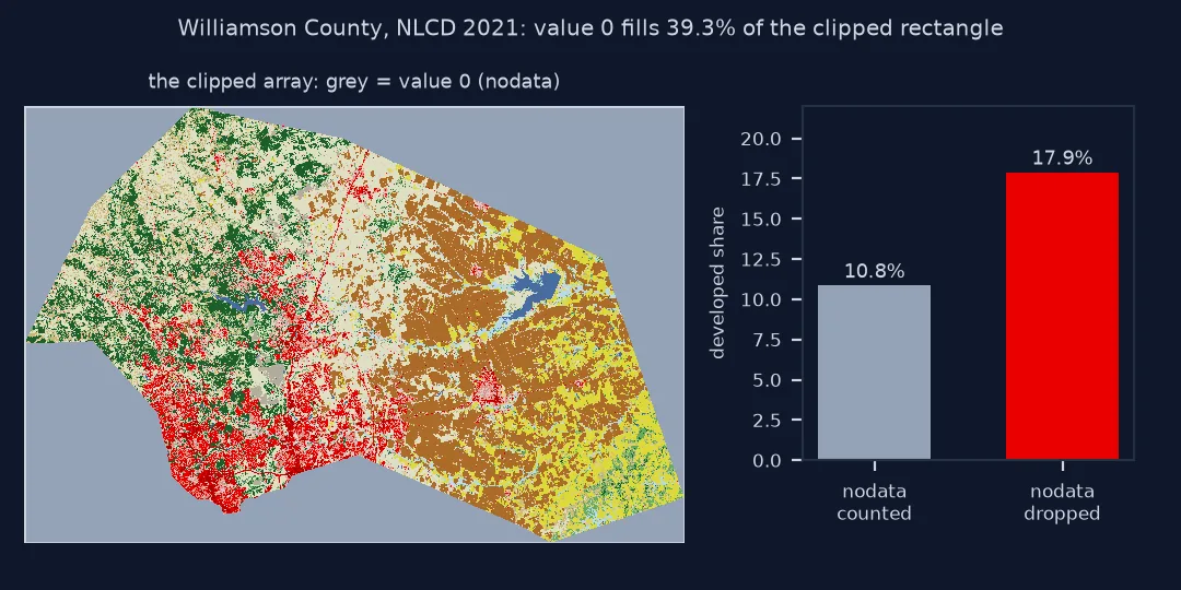
Williamson developed share, nodata counted: 10.8%; nodata dropped: 17.9%

Find the class that is not one, choose land or total area

1. Look for the class that is not a class

A masked raster keeps its rectangle. Count everything and the fill value shows up with the rest:

counted = shares(WILL, drop=())
print(f"value 0 holds {counted[0]:.1f}% of the array; the largest real class holds {counted.drop(0).max():.1f}%")
print(f"pixels in the rectangle: {WILL.size:,}; inside the county: {(WILL > 0).sum():,}")

value 0 holds 39.3% of the array; the largest real class holds 15.7%
pixels in the rectangle: 5,359,980; inside the county: 3,251,319

Any share computed over the rectangle is too small by the same factor, here the ratio of the rectangle to the county.

2. Choose land or total area

Water is a class too. For a statement about how much land is built on, divide by land:

water = [11, 12]
s = shares(MONT).reindex(range(256), fill_value=0)
print(f"Monterey County: water {s[water].sum():.1f}% of the mapped area; developed {s[dev].sum():.1f}% of the total, "
      f"{s[dev].sum() / (100 - s[water].sum()) * 100:.1f}% of the land")

Monterey County: water 0.7% of the mapped area; developed 4.9% of the total, 5.0% of the land

3. Mind the coast

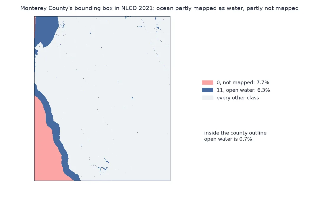
Beyond the coastline NLCD maps a strip of open water and then stops. In a coastal bounding box both appear:

box = shares(MONT_BOX, drop=())
print(f"Monterey bounding box: {box.get(0, 0):.1f}% unmapped (0), {box[11]:.1f}% open water (11)")
print(f"water share of the box with 0 dropped: {shares(MONT_BOX)[11]:.1f}%; inside the county outline: {shares(MONT)[11]:.1f}%")

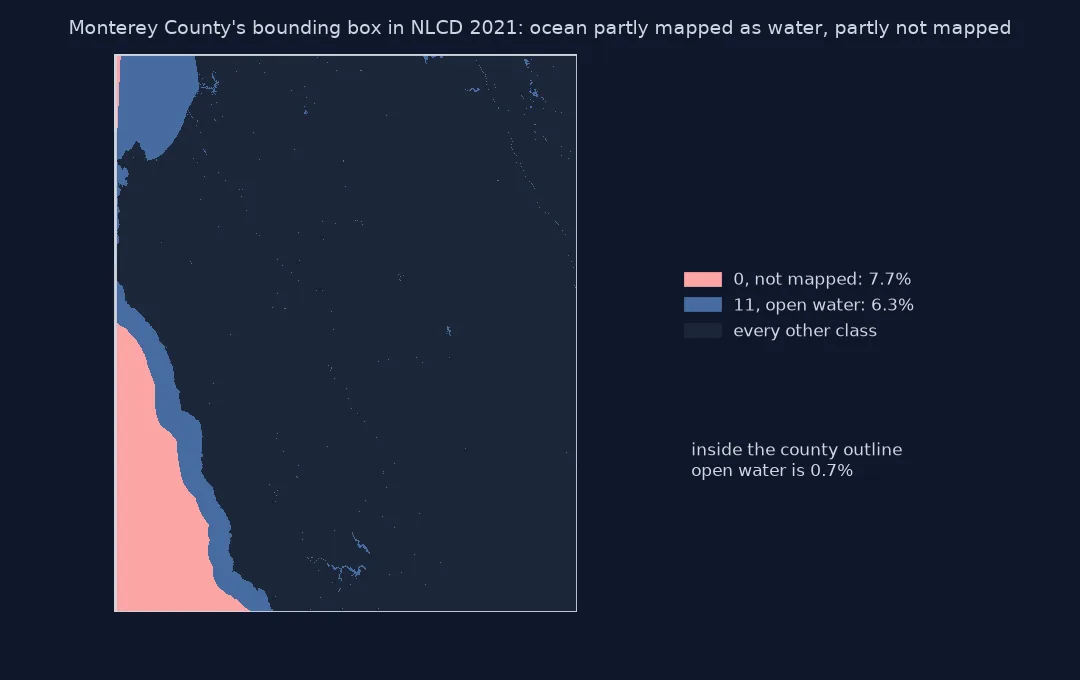
Monterey bounding box: 7.7% unmapped (0), 6.3% open water (11)
water share of the box with 0 dropped: 6.8%; inside the county outline: 0.7%

The box's water share is ten times the county's own, because most of that water is the Pacific.

A share function that refuses ambiguity

The data used on this page

NLCD 2021 (30 m) from MRLC's WCS for the bounding boxes of Williamson County, Texas, and Monterey County, California, masked with their 2023 Census cartographic boundary outlines. The WCS files declare 0 as nodata.

import time
from pathlib import Path

import geopandas as gpd
import numpy as np
import pandas as pd
import rasterio
import rasterio.mask
import requests

Path("data").mkdir(exist_ok=True)
if not Path("data/cb_2023_us_county_20m.zip").exists():
    Path("data/cb_2023_us_county_20m.zip").write_bytes(requests.get("https://www2.census.gov/geo/tiger/GENZ2023/shp/cb_2023_us_county_20m.zip", timeout=300).content)
counties = gpd.read_file("data/cb_2023_us_county_20m.zip").to_crs(5070)


def nlcd_for(geoid):
    county = counties[counties.GEOID == geoid]
    path = Path(f"data/nlcd_2021_{geoid}.tif")
    if not path.exists():
        x0, y0, x1, y1 = county.total_bounds
        for attempt in range(4):
            r = requests.get("https://www.mrlc.gov/geoserver/mrlc_download/wcs", params={"service": "WCS", "version": "2.0.1", "request": "GetCoverage",
                             "coverageId": "mrlc_download__NLCD_2021_Land_Cover_L48", "subset": [f"X({x0},{x1})", f"Y({y0},{y1})"], "format": "image/geotiff"}, timeout=300)
            if r.status_code < 500:
                break
            time.sleep(15 * (attempt + 1))
        r.raise_for_status()
        path.write_bytes(r.content)
    with rasterio.open(path) as src:
        box = src.read(1)
        masked = rasterio.mask.mask(src, county.geometry, crop=True, nodata=0)[0][0]
        nodata = src.nodata
    return box, masked, nodata


_, WILL, nd = nlcd_for("48491")
MONT_BOX, MONT, _ = nlcd_for("06053")
print(f"declared nodata: {nd}; Williamson array {WILL.shape[1]} x {WILL.shape[0]}; Monterey array {MONT.shape[1]} x {MONT.shape[0]}")

declared nodata: 0.0; Williamson array 2845 x 1884; Monterey array 4312 x 5201

Example 1: a share function that refuses ambiguity

def class_share(arr, classes, denominator="land", nodata=0, water=(11, 12)):
    valid = arr[arr != nodata]
    base = valid[~np.isin(valid, water)] if denominator == "land" else valid
    return np.isin(base, classes).mean() * 100

for name, arr in (("Williamson", WILL), ("Monterey", MONT)):
    print(f"{name}: developed {class_share(arr, dev, 'land'):.1f}% of land, {class_share(arr, dev, 'total'):.1f}% of the mapped total")

Williamson: developed 18.1% of land, 17.9% of the mapped total
Monterey: developed 5.0% of land, 4.9% of the mapped total

A raster is always a rectangle

A raster is always a rectangle. Clipping to a polygon cannot remove the corners, only mark them as nodata, and the mark is just a number. Functions such as np.unique, value_counts and histogram tools count every number unless told otherwise. The file's declared nodata value says which number to ignore; reading with masked=True, or dropping it explicitly as here, is what makes it count.

The denominator question is separate and just as consequential. "Share of the county" can mean the share of its mapped area, of its land, or of its official area including water. Here it hardly matters, because both county outlines follow the shore and hold little water; for counties around large lakes, reservoirs or bays it can matter. Neither choice is wrong, but percentages computed with different denominators cannot be compared.

Different nodata values and zero as data

• Different nodata values: some products use 255 or 250 for nodata or "outside"; read the file's nodata and the product documentation.
• When 0 is a value: in NLCD impervious surface, 0 means 0%; there, do not drop it (see impervious surface by watershed).
• Masked arrays: src.read(1, masked=True) hides the nodata value automatically; np.unique on the masked array's .compressed() then counts only valid pixels.
• All-touched masks include every pixel the boundary touches; the default uses pixel centres. Report which.
• Official areas (Census land and water area) will differ slightly from pixel counts because of boundary generalisation.

Internal links

• How to summarise land cover by polygon — shares by zone
• How to download NLCD land cover — the data

FAQ

Why do my land cover percentages add up to less than expected?

The nodata pixels outside your polygon are in the denominator. Drop the nodata value (usually 0) before counting.

Should land cover shares include water?

It depends on the question; for built-up or farmed land, divide by land area. State the denominator either way.

What is NLCD's nodata value?

In files from MRLC's WCS it is 0, which is not a land cover class.

How do I ignore nodata when counting raster values?

Read with masked=True and count arr.compressed(), or drop the nodata value from np.unique's result.