How to Measure Land Cover Around Points in Python

Problem statement

How green is the neighbourhood around each school, clinic, sensor or bird sighting? The usual answer is land cover composition in a buffer: the share of each class within 500 m or 1 km of the point. For one point it is a clip and a count. For hundreds of points the buffers overlap, and a zonal statistics run that rasterises all the buffers at once gives each overlapping pixel to only one of them, so crowded points lose part of their neighbourhood. Points near the edge of the downloaded raster lose part of theirs to the edge.

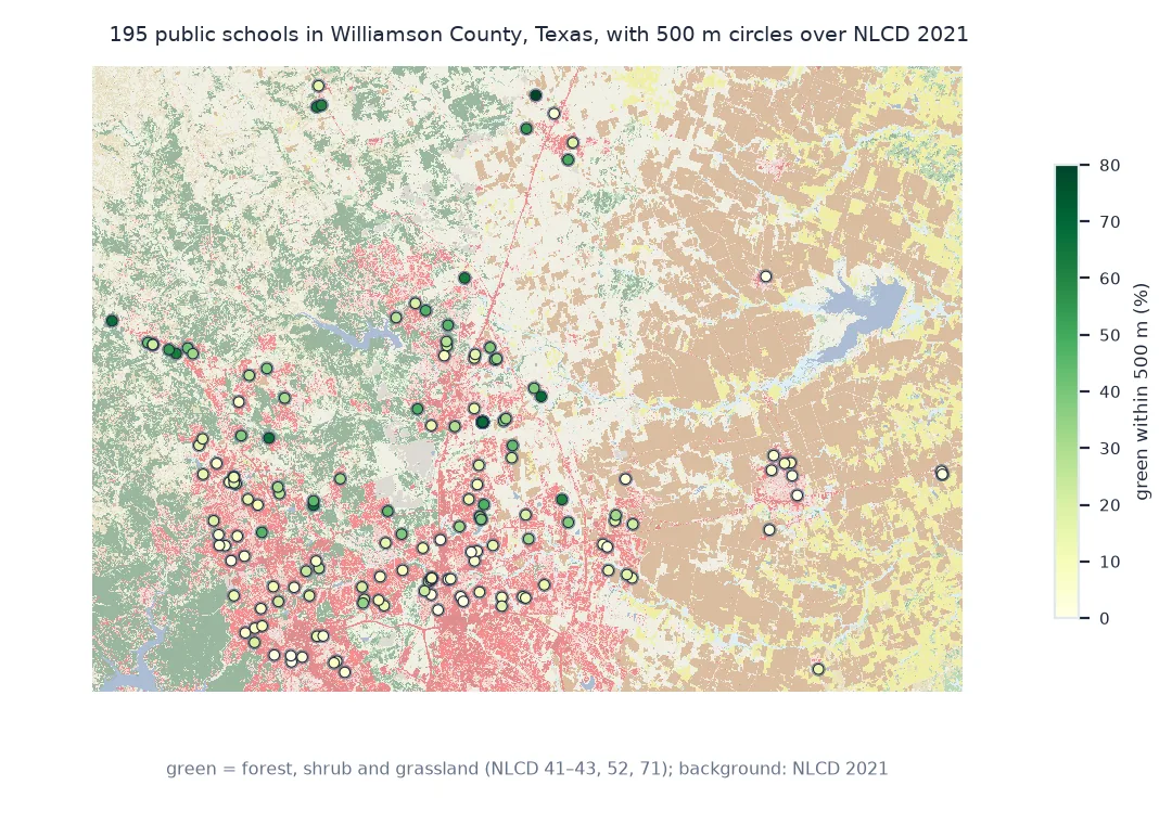
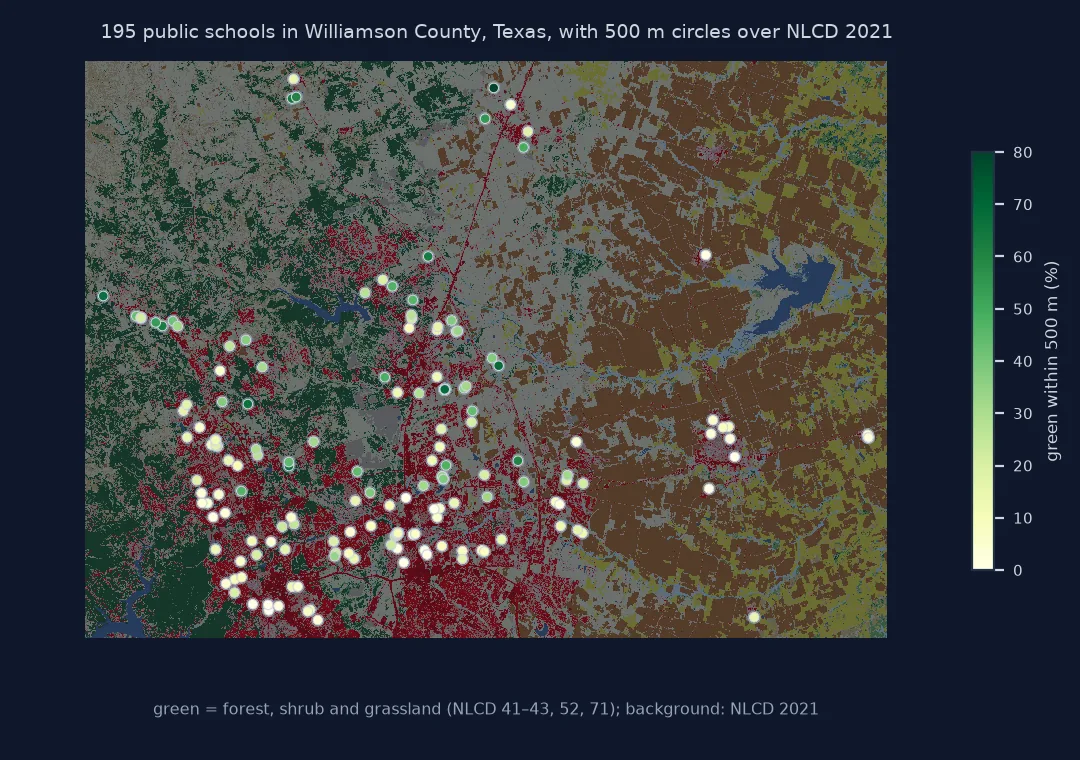
This page measures land cover within 500 m and 1 km of the 195 public schools in Williamson County, Texas, from NLCD 2021, one exact circle per school.

Quick answer

For each point, cut a window around it, keep the pixels whose centres fall within the radius, and count classes:

def composition(x, y, radius):
    col, row = ~TRANSFORM * (x, y)
    r = int(np.ceil(radius / 30)) + 1
    r0, c0 = int(row) - r, int(col) - r
    win = LC[r0:r0 + 2 * r + 1, c0:c0 + 2 * r + 1]
    yy, xx = np.mgrid[r0:r0 + win.shape[0], c0:c0 + win.shape[1]]
    px, py = TRANSFORM * (xx + 0.5, yy + 0.5)
    inside = (px - x) ** 2 + (py - y) ** 2 <= radius ** 2
    v = pd.Series(win[inside]).map(GROUP).value_counts(normalize=True) * 100
    return v.reindex(["Developed", "Green", "Agriculture", "Water"], fill_value=0)

comp = pd.DataFrame([composition(p.x, p.y, 500) for p in SCHOOLS.geometry], index=SCHOOLS.NAME)
print(f"{len(comp)} schools, 500 m radius: median {comp.Developed.median():.0f}% developed, {comp.Green.median():.0f}% green")
print(comp.Green.describe()[["min", "25%", "50%", "75%", "max"]].round(1).to_string())

195 schools, 500 m radius: median 76% developed, 18% green
min     0.0
25%     9.0
50%    18.2
75%    43.7
max    83.2

Pad the raster, keep buffers apart, compare radii

1. Pad the raster by the radius

A school near the county line needs land cover beyond it. Request the raster for the points' bounding box plus the largest radius, and check that every window fits:

x0, y0, x1, y1 = SCHOOLS.total_bounds
b = array_bounds(*LC.shape, TRANSFORM)
print(f"points span {x0:,.0f}–{x1:,.0f} m east; raster {b[0]:,.0f}–{b[2]:,.0f}; margin {min(x0 - b[0], b[2] - x1, y0 - b[1], b[3] - y1):,.0f} m")

points span -186,719–-123,928 m east; raster -188,205–-122,415; margin 1,486 m

2. Do not rasterise overlapping buffers together

Rasterising all buffers into one zone raster gives every pixel to the last buffer drawn over it. Count how much each school loses:

buffers = SCHOOLS.buffer(1000)
zones = features.rasterize([(g, k + 1) for k, g in enumerate(buffers)], out_shape=LC.shape, transform=TRANSFORM)
got = np.bincount(zones.ravel(), minlength=len(SCHOOLS) + 1)[1:]
full = np.pi * 1000 ** 2 / 900
print(f"1 km buffers: {(got < 0.9 * full).sum()} of {len(SCHOOLS)} schools keep under 90% of their pixels; worst keeps {got.min() / full:.0%}")
print(f"pairs of schools closer than 2 km: {int((SCHOOLS.geometry.apply(lambda p: (SCHOOLS.distance(p) < 2000).sum() - 1).sum()) / 2)}")
same = SCHOOLS.geometry.to_wkb().duplicated(keep=False)
print(f"{same.sum()} schools share their exact location with another, at {SCHOOLS[same].geometry.to_wkb().nunique()} sites")

1 km buffers: 123 of 195 schools keep under 90% of their pixels; worst keeps 0%
pairs of schools closer than 2 km: 788
47 schools share their exact location with another, at 7 sites

Several programmes, such as alternative and juvenile justice schools, are registered at the same address, so their buffers coincide exactly and all but one lose everything. Shared locations also weight a site several times in any average over schools; decide whether to count schools or sites.

3. Compare radii

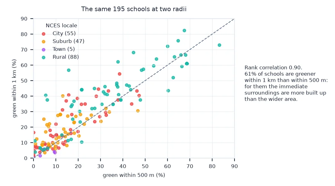
The answer depends on the radius; report it with every number:

comp1k = pd.DataFrame([composition(p.x, p.y, 1000) for p in SCHOOLS.geometry], index=SCHOOLS.NAME)
print(f"median green share: {comp.Green.median():.1f}% within 500 m, {comp1k.Green.median():.1f}% within 1 km")
print(f"rank correlation of green share between radii: {comp.Green.corr(comp1k.Green, method='spearman'):.2f}")

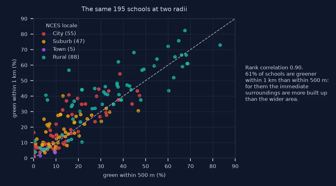
median green share: 18.2% within 500 m, 28.1% within 1 km
rank correlation of green share between radii: 0.90

Green space around schools by locale

The data used on this page

Public school locations for 2022–23 from the National Center for Education Statistics EDGE program (public ArcGIS service), filtered to Williamson County, Texas, and NLCD 2021 (30 m) from MRLC's WCS for the schools' bounding box padded by 1.5 km, in CONUS Albers (EPSG:5070).

import time
from pathlib import Path

import geopandas as gpd
import numpy as np
import pandas as pd
import rasterio
import requests
from rasterio import features
from rasterio.transform import array_bounds

Path("data").mkdir(exist_ok=True)
NCES = "https://nces.ed.gov/opengis/rest/services/K12_School_Locations/EDGE_GEOCODE_PUBLICSCH_2223/MapServer/0/query"
SCHOOLS = gpd.read_file(requests.get(NCES, params={"where": "STATE = 'TX' AND NMCNTY = 'Williamson County'",
                                                   "outFields": "NAME,LOCALE,CITY", "outSR": 4326, "f": "geojson"}, timeout=120).text).to_crs(5070)
x0, y0, x1, y1 = SCHOOLS.total_bounds + np.array([-1500, -1500, 1500, 1500])
path = Path("data/nlcd_2021_schools.tif")
if not path.exists():
    WCS = "https://www.mrlc.gov/geoserver/mrlc_download/wcs"
    for attempt in range(4):
        r = requests.get(WCS, params={"service": "WCS", "version": "2.0.1", "request": "GetCoverage", "coverageId": "mrlc_download__NLCD_2021_Land_Cover_L48",
                                      "subset": [f"X({x0},{x1})", f"Y({y0},{y1})"], "format": "image/geotiff"}, timeout=300)
        if r.status_code < 500:
            break
        time.sleep(15 * (attempt + 1))
    r.raise_for_status()
    path.write_bytes(r.content)
with rasterio.open(path) as src:
    LC, TRANSFORM = src.read(1), src.transform
GROUP = {11: "Water", 90: "Water", 95: "Water", 21: "Developed", 22: "Developed", 23: "Developed", 24: "Developed",
         41: "Green", 42: "Green", 43: "Green", 52: "Green", 71: "Green", 31: "Barren", 81: "Agriculture", 82: "Agriculture"}
print(f"{len(SCHOOLS)} schools; NLCD window {LC.shape[1]} x {LC.shape[0]} pixels")

195 schools; NLCD window 2193 x 1580 pixels

Example 1: green space by NCES locale

locale = SCHOOLS.LOCALE.astype(str).str[0].map({"1": "City", "2": "Suburb", "3": "Town", "4": "Rural"})
print(comp.Green.groupby(locale.values).agg(["count", "median"]).round(1).to_string())

        count  median
City       55    10.2
Rural      88    46.3
Suburb     47    12.0
Town        5     4.6

The median rural school has 46% green land within 500 m; city and suburban schools have 10–12%.

Circular zones that overlap

A buffer composition is a categorical zonal summary with circular zones. When zones do not overlap, rasterising them all at once and cross-tabulating is efficient. Points that serve neighbourhoods, such as schools, cluster, and their buffers overlap heavily, so each one must be summarised on its own: either by masking a window per point, as here, or by running the zonal step once per buffer. A circle traced on 30 m pixels holds about 873 pixels at 500 m, enough that pixel-centre membership is a fine approximation.

The radius is part of the definition. A 500 m buffer describes what is within a short walk, 1 km the wider neighbourhood. Shares at different radii are correlated but not interchangeable, and published studies of greenness and health differ partly because they chose different radii and different definitions of "green". Here green means forest, shrub and grassland; parks mapped as developed open space (class 21) are not counted, a choice worth stating.

Projected buffers, padding and point accuracy

• Projected CRS: compute buffers and distances in metres; EPSG:5070 here.
• Edge padding: pad the raster by at least the largest radius, or points near the edge get truncated circles.
• Class definitions: decide whether developed open space counts as green; it holds most urban parks and lawns in NLCD.
• Point accuracy: geocoded school locations are usually the building or the parcel; a 30 m error barely changes a 500 m composition.
• Many points: for thousands of points, process windows in a loop as here, or use exactextract with one feature per buffer.

Internal links

• How to summarise land cover by polygon — non-overlapping zones
• How to reclassify a land cover raster — building groups such as "green"

FAQ

How do I calculate land cover in a buffer around points in Python?

For each point, read a window of the raster around it, keep the pixels whose centres lie within the radius, and count the classes.

Why do my buffer statistics change when buffers overlap?

Rasterising overlapping buffers into one zone layer gives each pixel to one buffer only, so overlapping buffers lose pixels. Summarise each buffer separately.

What buffer radius should I use?

It depends on the question: about 300–500 m for what is within a short walk, 1 km or more for neighbourhood context. Report the radius and test whether results change with it.

Does NLCD count parks as green space?

Many urban parks are mapped as developed open space (class 21), not as forest or grassland.