How to Reclassify a Land Cover Raster in Python

On this page

Problem statement

Land cover products come with more classes than most analyses need. NLCD has 16, including four intensities of developed land and three kinds of forest, and a study of urban expansion or habitat often wants five or six broad groups. Reclassifying means mapping every input code to an output code. Done carelessly, it silently drops classes that were not in the mapping, leaves unmapped pixels with their old codes so they masquerade as new classes, or runs a Python function per pixel, which here is about 50 times slower than it needs to be.

This page reclassifies NLCD 2021 for Williamson County, Texas (5.4 million pixels in its bounding box) into six groups with a lookup table. It checks that every code was mapped, times the common alternatives, and writes the result with its own colour table.

Quick answer

Build a 256-entry lookup table indexed by the input code and index it with the raster:

lut = np.full(256, 255, dtype=np.uint8)                      # 255 = "not in the crosswalk"
for code, group in CROSSWALK.items():
    lut[code] = group
lut[0] = 0                                                   # keep nodata as nodata
grouped = lut[LC]
print(f"{LC.size:,} pixels reclassified; unmapped pixels: {(grouped == 255).sum()}")
print(pd.Series(grouped[grouped > 0]).map(GROUP_NAMES).value_counts().to_string())

5,359,980 pixels reclassified; unmapped pixels: 0
Shrub and grass      1027598
Agriculture          1013282
Developed             581313
Forest                483859
Water and wetland     108296
Barren                 36971

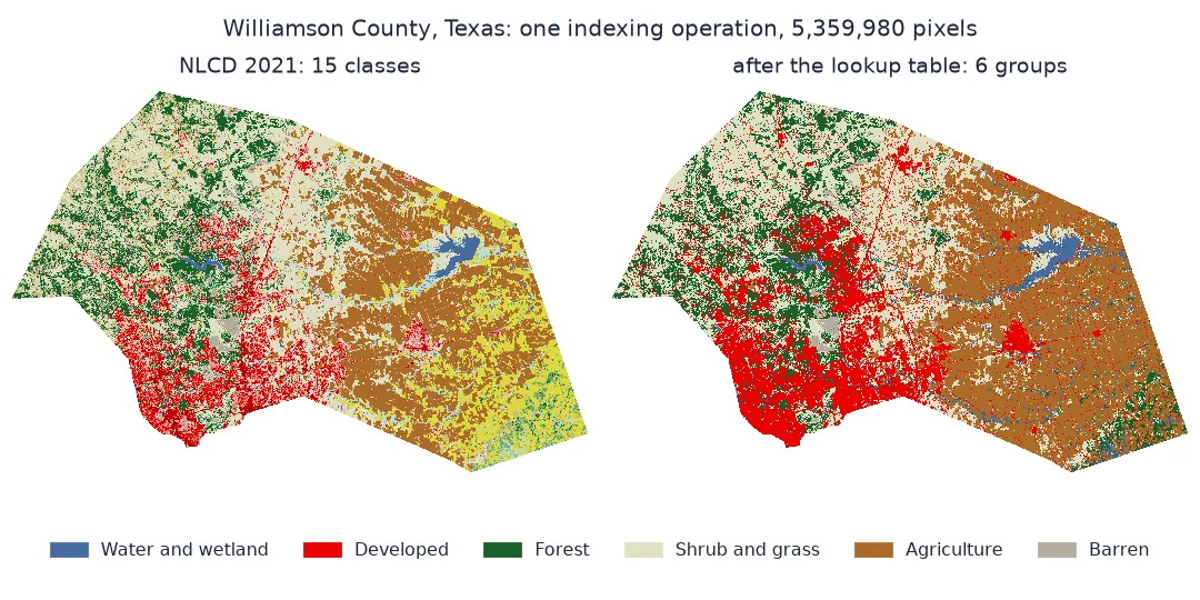
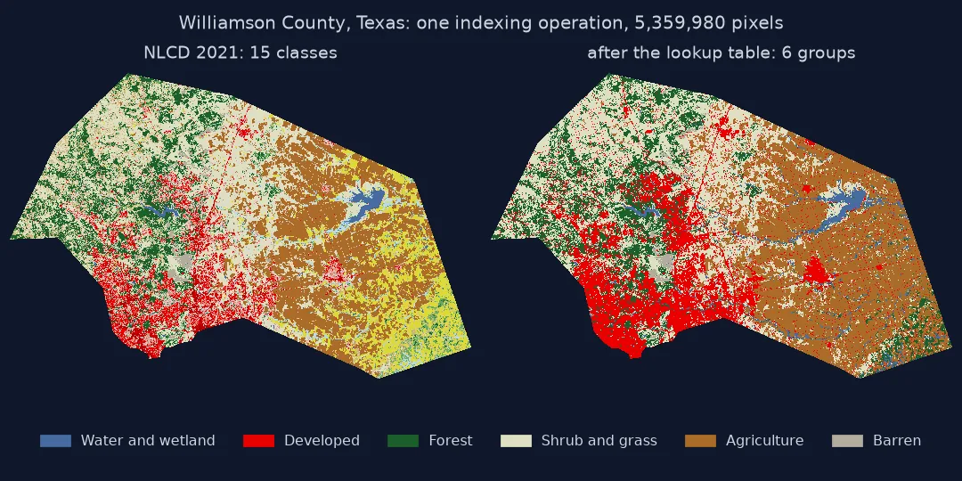
Two maps of Williamson County, Texas: on the left NLCD 2021 in its 15 classes present, on the right the same pixels after the lookup table in six groups, developed in red, forest in green, shrub and grass in pale beige, agriculture in brown, water and wetland in blue and barren in grey. — Sixteen NLCD classes to six groups in one indexing operation.

A crosswalk that covers every code, compared methods, colours

1. Check the crosswalk covers every code present

A crosswalk written from the legend can miss codes that appear in the data, and one written from one area can miss codes another area has:

present = {int(c) for c in np.unique(LC)} - {0}
print("codes present:", sorted(present))
print("codes present but not in the crosswalk:", sorted(present - set(CROSSWALK)) or "none")
print("crosswalk codes absent here:", sorted(set(CROSSWALK) - present) or "none")

codes present: [11, 21, 22, 23, 24, 31, 41, 42, 43, 52, 71, 81, 82, 90, 95]
codes present but not in the crosswalk: none
crosswalk codes absent here: [12]

Sending unmapped codes to a sentinel value (255 here) makes a gap visible. With np.select or a dictionary get with a default, the default decides what an unmapped code becomes, so choose one that cannot be mistaken for a class.

2. Compare the methods

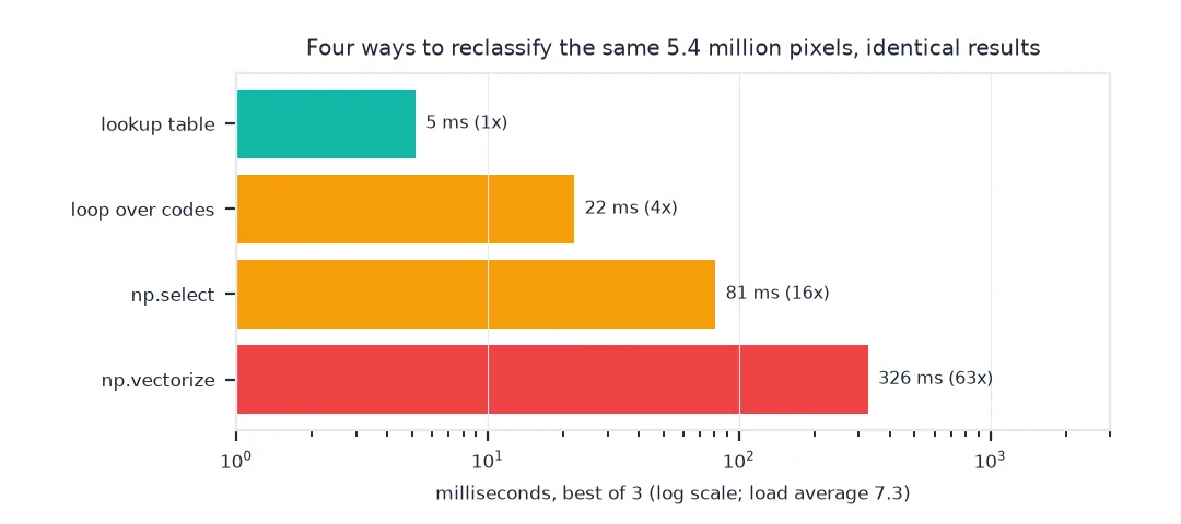
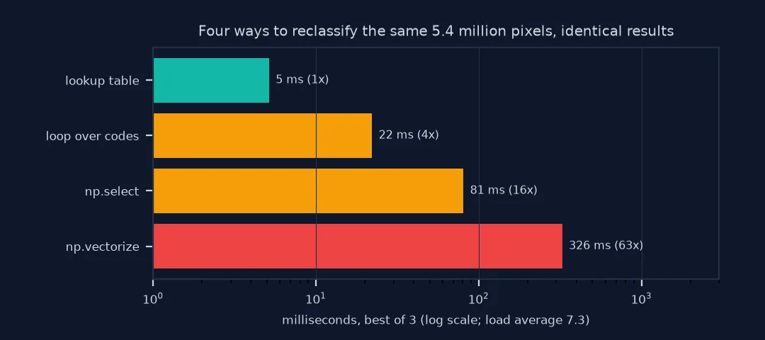
All four common approaches give the same answer; they differ in speed:

def by_vectorize(a):
    return np.vectorize(lambda v: CROSSWALK.get(int(v), 255 if v else 0), otypes=[np.uint8])(a)

def by_select(a):
    conds = [np.isin(a, [c for c, g in CROSSWALK.items() if g == k]) for k in GROUP_NAMES]
    return np.select(conds, list(GROUP_NAMES), default=0).astype(np.uint8)

def by_loop(a):
    out = np.zeros_like(a)
    for code, group in CROSSWALK.items():
        out[a == code] = group
    return out

results = {}
for name, f in (("lookup table", lambda a: lut[a]), ("loop over codes", by_loop), ("np.select", by_select), ("np.vectorize", by_vectorize)):
    t0 = time.perf_counter(); out = f(LC); results[name] = time.perf_counter() - t0
    assert (out == grouped).all()
print(f"load average {os.getloadavg()[0]:.1f}; seconds for {LC.size:,} pixels:", {k: round(v, 3) for k, v in results.items()})

load average 3.5; seconds for 5,359,980 pixels: {'lookup table': 0.006, 'loop over codes': 0.025, 'np.select': 0.078, 'np.vectorize': 0.319}

The lookup table touches each pixel once. The loop and np.select scan the whole raster once per class; np.vectorize calls a Python function per pixel.

Bar chart on a logarithmic scale of time to reclassify 5.4 million pixels: lookup table about 5 milliseconds, loop over codes about 22, np.select about 81 and np.vectorize about 326, roughly 60 times the lookup table; all four give identical results. — Same output, very different cost.

3. Write the result with its own colours

A reclassified raster needs its own palette, or viewers will paint group 3 with whatever colour code 3 had:

profile.update(dtype="uint8", nodata=0, compress="deflate")
with rasterio.open("data/williamson_groups.tif", "w", **profile) as dst:
    dst.write(grouped, 1)
    dst.write_colormap(1, {k: tuple(int(GROUP_COLORS[k][i:i + 2], 16) for i in (1, 3, 5)) + (255,) for k in GROUP_NAMES})
    dst.update_tags(1, **{f"class_{k}": v for k, v in GROUP_NAMES.items()})
with rasterio.open("data/williamson_groups.tif") as src:
    print(src.colormap(1)[3], src.tags(1)["class_3"])

(28, 95, 44, 255) Forest

Areas survive reclassification

The data used on this page

NLCD 2021 (2021 release, 30 m) for Williamson County, Texas, from MRLC's WCS, masked to the 2023 Census county outline.

import os
import time
from pathlib import Path

import geopandas as gpd
import numpy as np
import pandas as pd
import rasterio
import rasterio.mask
import requests

Path("data").mkdir(exist_ok=True)
WCS = "https://www.mrlc.gov/geoserver/mrlc_download/wcs"
if not Path("data/cb_2023_us_county_20m.zip").exists():
    Path("data/cb_2023_us_county_20m.zip").write_bytes(requests.get("https://www2.census.gov/geo/tiger/GENZ2023/shp/cb_2023_us_county_20m.zip", timeout=300).content)
COUNTY = gpd.read_file("data/cb_2023_us_county_20m.zip").query("GEOID == '48491'").to_crs(5070)
path = Path("data/nlcd_2021.tif")
if not path.exists():
    x0, y0, x1, y1 = COUNTY.total_bounds
    for attempt in range(4):
        r = requests.get(WCS, params={"service": "WCS", "version": "2.0.1", "request": "GetCoverage", "coverageId": "mrlc_download__NLCD_2021_Land_Cover_L48",
                                      "subset": [f"X({x0},{x1})", f"Y({y0},{y1})"], "format": "image/geotiff"}, timeout=300)
        if r.status_code < 500:
            break
        time.sleep(15 * (attempt + 1))
    r.raise_for_status()
    path.write_bytes(r.content)
with rasterio.open(path) as src:
    lc, tr = rasterio.mask.mask(src, COUNTY.geometry, crop=True, nodata=0)
    profile = src.profile | {"height": lc.shape[1], "width": lc.shape[2], "transform": tr}
LC = lc[0]
GROUP_NAMES = {1: "Water and wetland", 2: "Developed", 3: "Forest", 4: "Shrub and grass", 5: "Agriculture", 6: "Barren"}
GROUP_COLORS = {1: "#466b9f", 2: "#eb0000", 3: "#1c5f2c", 4: "#dfdfc2", 5: "#ab6c28", 6: "#b3ac9f"}
CROSSWALK = {11: 1, 12: 1, 90: 1, 95: 1, 21: 2, 22: 2, 23: 2, 24: 2, 41: 3, 42: 3, 43: 3, 52: 4, 71: 4, 81: 5, 82: 5, 31: 6}
print(f"{LC.shape[1]} x {LC.shape[0]} pixels, {(LC > 0).sum():,} inside the county; {len(CROSSWALK)} codes into {len(GROUP_NAMES)} groups")

2845 x 1884 pixels, 3,251,319 inside the county; 16 codes into 6 groups

Example 1: areas survive reclassification

before = pd.Series(LC[LC > 0]).map(CROSSWALK).value_counts().sort_index() * 900 / 1e6
after = pd.Series(grouped[grouped > 0]).value_counts().sort_index() * 900 / 1e6
print(pd.DataFrame({"group": [GROUP_NAMES[k] for k in after.index], "km² before": before.values, "km² after": after.values}).round(1).to_string(index=False))

            group  km² before  km² after
Water and wetland        97.5       97.5
        Developed       523.2      523.2
           Forest       435.5      435.5
  Shrub and grass       924.8      924.8
      Agriculture       912.0      912.0
           Barren        33.3       33.3

Reclassification is a lookup table

Reclassification is a function from input codes to output codes, applied to every pixel. Land cover codes are small integers, so the function can be stored as an array indexed by the code and applied with one indexing operation. NumPy does that in a single pass in compiled code, which is why the lookup table is the fastest method and, with a sentinel for unmapped codes, also the safest.

The crosswalk is a modelling choice: write it down.

Two things are easy to forget. The crosswalk is a modelling choice: whether shrubland belongs with grassland, whether pasture is agriculture or grassland, whether open space counts as developed. Write it down with the output. And the output is a new product, with new codes, so it needs its own colour table and class names; reusing the input's palette paints the new codes with colours meant for something else.

16-bit codes, floats and nodata

Reclassification problems and fixes.

Codes above 255: for 16-bit products, size the table to the largest code plus one, or use np.searchsorted on sorted codes.
Float rasters: reclassify continuous values with np.digitize on bin edges instead.
Nodata: map the input nodata explicitly; here 0 stays 0.
rasterio/xarray: xr.apply_ufunc(lambda a: lut[a], da) applies the same table lazily to large arrays.
Timings depend on the machine and its load; the ranking does not.

Internal links

How to summarise land cover by polygon — grouping counts after the fact
How to download NLCD land cover — the data

FAQ

How do I reclassify a raster in Python?

Build a lookup table indexed by the old codes (lut[old] = new), then index it with the raster: new = lut[raster].

What is the fastest way to reclassify land cover in NumPy?

A lookup table. It touches each pixel once; loops and np.select scan the raster once per class, and np.vectorize calls Python for every pixel.

How do I find codes missing from my reclassification?

Compare np.unique(raster) with the crosswalk's keys, and map unknown codes to a sentinel value so they show up.

Do I need a new colour table after reclassifying?

Yes. The output codes are new classes; write a colour map and class names for them.