
Land Cover Map Accuracy Explained
On this page
Problem statement
Every land cover map comes with an overall accuracy figure, and every user of the map quietly assumes it applies evenly. It does not. Overall accuracy averages over classes that are mapped very well and classes that are mapped poorly. It says nothing about whether a class's area is too large or too small. And it depends on how the reference sample was chosen. Reading a map properly means reading its confusion matrix: user's and producer's accuracy per class, and what the errors do to areas.
This page compares ESA WorldCover 2020 with 667 field-surveyed points of the EU's LUCAS 2018 Copernicus survey in Denmark. It computes the standard accuracy measures and shows what each one means for someone using the map.
Quick answer
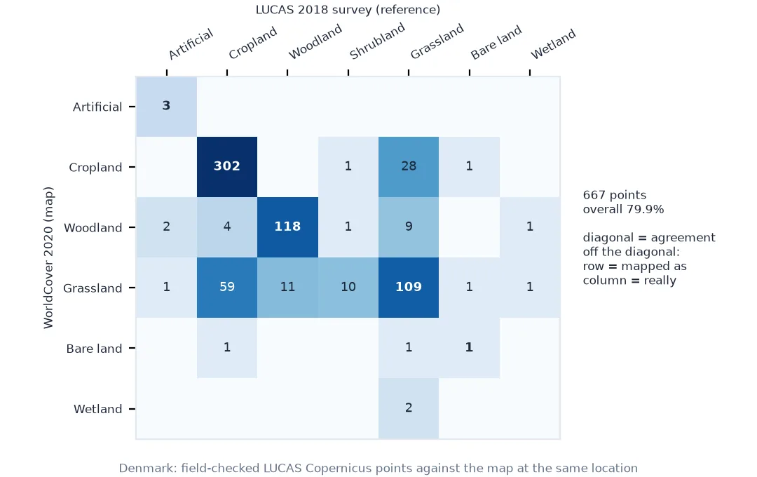
Sample the map at the reference points, put both in the same classes, and cross-tabulate:
cm = pd.crosstab(PTS.mapped, PTS.ref)
overall = np.trace(cm.reindex(index=cm.columns, fill_value=0).to_numpy()) / cm.to_numpy().sum()
print(cm.rename(index=NAMES, columns=NAMES).to_string())
print(f"overall accuracy: {overall:.1%} of {len(PTS)} points")
ref Artificial Cropland Woodland Shrubland Grassland Bare land Wetland
mapped
Artificial 3 0 0 0 0 0 0
Cropland 0 302 0 1 28 1 0
Woodland 2 4 118 1 9 0 1
Grassland 1 59 11 10 109 1 1
Bare land 0 1 0 0 1 1 0
Wetland 0 0 0 0 2 0 0
overall accuracy: 79.9% of 667 points
User's and producer's accuracy, off-diagonal cells, area effects
1. User's and producer's accuracy
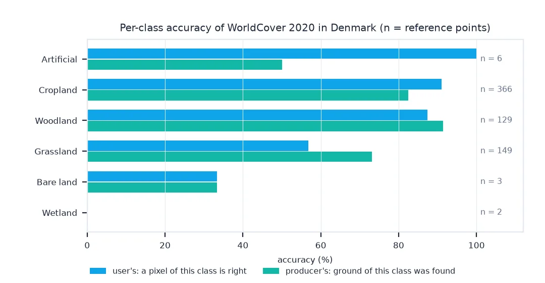
Rows are what the map says, columns what the surveyor found. User's accuracy, along a row, is the chance that a pixel mapped as a class really is that class: what a user of the map experiences. Producer's accuracy, down a column, is the chance that ground of a class was mapped as that class: how well the producer captured it.
classes = [c for c in cm.columns if c in cm.index]
acc = pd.DataFrame({"mapped": [cm.loc[c].sum() for c in classes], "reference": [cm[c].sum() for c in classes],
                    "user's": [cm.loc[c, c] / cm.loc[c].sum() for c in classes],
                    "producer's": [cm.loc[c, c] / cm[c].sum() for c in classes]}, index=[NAMES[c] for c in classes])
print(acc.round(2).to_string())
mapped reference user's producer's
Artificial 3 6 1.00 0.50
Cropland 332 366 0.91 0.83
Woodland 135 129 0.87 0.91
Grassland 192 149 0.57 0.73
Bare land 3 3 0.33 0.33
Wetland 2 2 0.00 0.00
Classes with a handful of points (built-up, bare, wetland here) have accuracies that mean little; with 3 points, one error moves the figure by a third.
2. Read the off-diagonal cells
The errors are not random. Find the largest:
off = cm.stack()
off = off[[m != r for m, r in off.index]].sort_values(ascending=False).head(4)
for (m, r), n in off.items():
    print(f"{n:3d} points surveyed as {NAMES[r]} but mapped as {NAMES[m]}")
crop_as_grass = PTS[(PTS.mapped == "E") & (PTS.ref == "B")]
print("what the surveyors recorded there:", crop_as_grass.LC1_LABEL.value_counts().head(3).to_dict())
59 points surveyed as Cropland but mapped as Grassland
28 points surveyed as Grassland but mapped as Cropland
11 points surveyed as Woodland but mapped as Grassland
10 points surveyed as Shrubland but mapped as Grassland
what the surveyors recorded there: {'Barley': 28, 'Temporary grasslands': 9, 'Common wheat': 5}
Grassland and cropland swap in both directions, and most of the cropland mapped as grass is cereal fields, barley above all. A cereal field is green, grass-like vegetation for much of the year, and a map with one label per year has to choose; temporary grass in rotation, which surveyors record as a crop, adds to the confusion. The classes are defined from different evidence.
3. See what errors do to area
When errors in one direction outnumber errors in the other, the mapped area of a class is biased. With the map's class proportions as weights, the reference proportions can be estimated from the matrix:
W = MAP_SHARE.reindex(cm.index).fillna(0)                          # share of Denmark's land in each mapped class
P = cm.div(cm.sum(axis=1), axis=0).mul(W, axis=0)                  # estimated share of land in (map row, reference column)
est = P.sum(axis=0)
compare = pd.DataFrame({"mapped share": W, "estimated true share": est}).reindex(classes).rename(NAMES) * 100
print(compare.round(1).to_string())
mapped share estimated true share
Artificial 2.3 2.7
Cropland 46.9 52.6
Woodland 19.6 18.8
Grassland 30.3 23.2
Bare land 0.3 0.4
Wetland 0.7 0.3
The map shares come from the 1:16 overview of the map, about 150 m, which under-counts scattered classes such as buildings. This is the stratified estimator of Olofsson and colleagues (2014). It is only valid when the reference points are a probability sample of the map, which these are not quite: LUCAS Copernicus points were surveyed where the land cover is homogeneous for some tens of metres. Treat the result as an illustration of the method, not a corrected map of Denmark.
How certain the overall accuracy is
The data used on this page
LUCAS 2018 Copernicus in-situ land cover from the EU Joint Research Centre (d'Andrimont et al. 2021), points marked COPERNICUS_CLEANED in Denmark with their level-1 Copernicus land cover; ESA WorldCover 2020 (v100) sampled at the theoretical point locations from the public S3 bucket; Denmark's outline from geoBoundaries.
import io
import zipfile
from pathlib import Path

import geopandas as gpd
import numpy as np
import pandas as pd
import rasterio
import rasterio.features
import requests
from rasterio.enums import Resampling

Path("data").mkdir(exist_ok=True)
Z = Path("data/LUCAS_2018_Copernicus.zip")
if not Z.exists():
    Z.write_bytes(requests.get("https://jeodpp.jrc.ec.europa.eu/ftp/jrc-opendata/LUCAS/LUCAS_2018_Copernicus.zip", timeout=600).content)
cols = ["POINT_ID", "NUTS0", "TH_LAT", "TH_LONG", "CPRN_LC", "LC1", "LC1_LABEL", "COPERNICUS_CLEANED"]
lucas = pd.read_csv(zipfile.ZipFile(Z).open("LUCAS_2018_Copernicus_attributes.csv"), usecols=cols, low_memory=False)
PTS = lucas[(lucas.NUTS0 == "DK") & lucas.COPERNICUS_CLEANED].copy()
WC = "https://esa-worldcover.s3.eu-central-1.amazonaws.com/v100/2020/map/ESA_WorldCover_10m_2020_v100_{}_Map.tif"
tile = lambda lat, lon: f"N{int(np.floor(lat / 3) * 3):02d}E{int(np.floor(lon / 3) * 3):03d}"
PTS["tile"] = [tile(a, b) for a, b in zip(PTS.TH_LAT, PTS.TH_LONG)]
values = {}
for t, g in PTS.groupby("tile"):
    with rasterio.open("/vsicurl/" + WC.format(t)) as src:
        values.update({pid: int(v[0]) for pid, v in zip(g.POINT_ID, src.sample(list(zip(g.TH_LONG, g.TH_LAT))))})
WC2LUCAS = {10: "C", 20: "D", 30: "E", 40: "B", 50: "A", 60: "F", 70: "F", 80: "G", 90: "H", 95: "H", 100: "E"}
PTS["mapped"] = PTS.POINT_ID.map(values).map(WC2LUCAS)
PTS["ref"] = PTS.CPRN_LC.str[0]
NAMES = {"A": "Artificial", "B": "Cropland", "C": "Woodland", "D": "Shrubland", "E": "Grassland", "F": "Bare land", "G": "Water", "H": "Wetland"}
DK = Path("data/dnk_adm0.geojson")
if not DK.exists():
    DK.write_bytes(requests.get("https://github.com/wmgeolab/geoBoundaries/raw/9469f09/releaseData/gbOpen/DNK/ADM0/geoBoundaries-DNK-ADM0_simplified.geojson", timeout=300).content)
dk = gpd.read_file(DK)
counts = pd.Series(0.0, index=list(NAMES))
for t in sorted(PTS.tile.unique()):
    with rasterio.open("/vsicurl/" + WC.format(t)) as src:              # read the 1:16 overview, about 150 m pixels
        ov = src.read(1, out_shape=(src.height // 16, src.width // 16), resampling=Resampling.nearest)
        ovt = src.transform * src.transform.scale(16, 16)
    inside = rasterio.features.geometry_mask(dk.geometry, ov.shape, ovt, invert=True)
    lat = ovt.f + (np.arange(ov.shape[0]) + 0.5) * ovt.e
    w = np.cos(np.radians(lat))[:, None] * np.ones_like(ov, dtype=float)    # pixel area shrinks with latitude
    for code, cls in WC2LUCAS.items():
        counts[cls] += w[inside & (ov == code)].sum()
land = counts.drop("G")
MAP_SHARE = land / land.sum()
print(f"{len(PTS)} LUCAS points in Denmark; WorldCover sampled at all: {PTS.mapped.notna().all()}; tiles {sorted(PTS.tile.unique())}")
667 LUCAS points in Denmark; WorldCover sampled at all: True; tiles ['N54E006', 'N54E009', 'N54E012', 'N57E006', 'N57E009']
Example 1: how certain is the overall accuracy?
n = len(PTS); se = np.sqrt(overall * (1 - overall) / n)
print(f"overall accuracy {overall:.1%} ± {1.96 * se:.1%} (95% interval, {n} points)")
print(f"grassland user's accuracy {acc.loc['Grassland', "user's"]:.0%} ± {1.96 * np.sqrt(acc.loc['Grassland', "user's"] * (1 - acc.loc['Grassland', "user's"]) / cm.loc['E'].sum()):.0%}")
overall accuracy 79.9% ± 3.0% (95% interval, 667 points)
grassland user's accuracy 57% ± 7%
What a confusion matrix compares
A confusion matrix compares a map with reference observations at the same places. Its diagonal is agreement; everything else is error, and the position of each error says which way it goes. Overall accuracy adds up the diagonal and hides the structure. User's accuracy tells a map user how far to trust a pixel of a given class. Producer's accuracy tells how much of the real class the map found. A class can score well on one and badly on the other: here grassland is found fairly well but over-mapped, so a grassland pixel is right only about three times in five.
Accuracy figures are only as good as the reference sample. Points must be independent of the map, labelled with the same class definitions, and chosen by a known random design, so that each point's weight in the estimate is known. Field surveys such as LUCAS are the best available reference in Europe, but their class definitions (land use mixed into cover) and point selection differ from the map's. Errors measured with them combine map errors with these differences, which is why published accuracies vary so much between assessments of the same map.
Location error, time and small classes
- Location error: a point near a class boundary can fall on either side of it; LUCAS Copernicus chose homogeneous surroundings partly to reduce this.
- Time: the survey is from 2018 and the map from 2020; real change in between counts as error.
- Crosswalks: mapping WorldCover classes onto LUCAS letters is a choice, and moss and lichen (WorldCover 100) has no clean equivalent.
- Water: lakes and sea are excluded here as reference points are on land; the map shares are land-only for that reason.
- Small classes: report the number of reference points beside every per-class accuracy.
Internal links
- Land cover products explained — what each map was designed for
- Why is my land cover change map full of speckle? — what map errors do to change
FAQ
What is the difference between user's and producer's accuracy?
User's accuracy is the share of pixels mapped as a class that really are that class; producer's accuracy is the share of the real class that was mapped as it.
Is overall accuracy enough to judge a land cover map?
No. It averages over classes; a map can be 80% accurate overall and much less reliable for the class you care about.
Can I correct land cover areas for map errors?
Yes, with the stratified estimator of Olofsson et al. (2014), if the reference sample is a probability sample of the map.
Where can I find reference data to check a land cover map?
In Europe, the LUCAS survey; elsewhere, validation datasets published with global maps, or a sample interpreted from high-resolution imagery.