How to Analyse a Land Cover Time Series in Python

On this page

Problem statement

Two land cover maps give a before and after. A series of nine gives a history: when each place changed, how often, and whether a change stuck. That needs the maps stacked into one three-dimensional array, years by rows by columns, and summaries along the time axis: class areas per year, the number of changes per pixel, the year of the last change. Done naively it means nine full rasters in memory and loops over pixels; done with NumPy it is a few vectorised operations.

This page stacks the nine NLCD years from 2001 to 2021 for Williamson County, Texas, and summarises the 3.25 million pixels' histories.

Quick answer

Stack the years into one array and compute along the first axis:

STACK = np.stack([LC[y] for y in YEARS])                      # (9, rows, cols), uint8
valid = (STACK > 0).all(axis=0)
G = LUT[STACK]                                                # reclassify all nine years at once
changes = (G[1:] != G[:-1]).sum(axis=0)                       # group changes per pixel between consecutive years
print(f"stack {STACK.shape}, {STACK.nbytes / 1e6:.0f} MB; pixels: {valid.sum():,}")
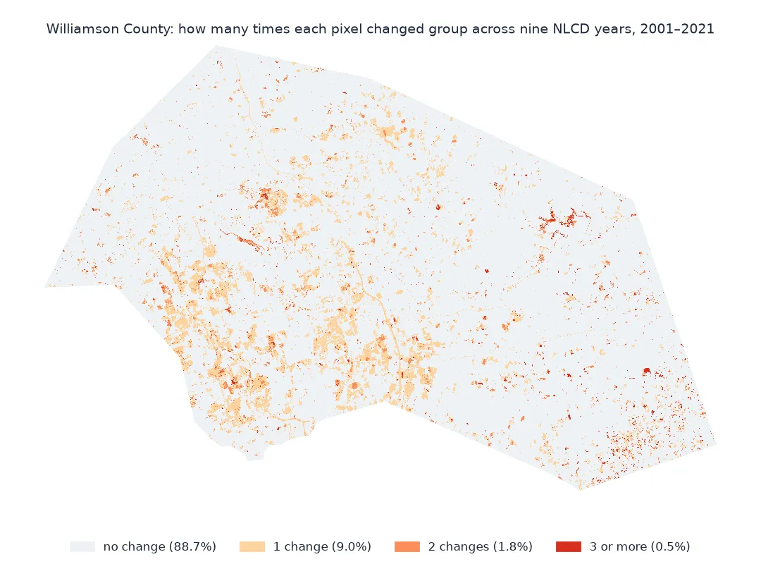
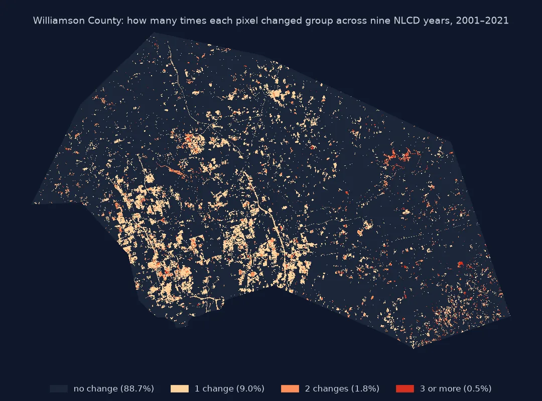
print("pixels by number of group changes:", {int(k): f"{v:.2%}" for k, v in
      pd.Series(changes[valid]).value_counts(normalize=True).sort_index().items()})

stack (9, 1884, 2845), 48 MB; pixels: 3,251,319
pixels by number of group changes: {0: '88.66%', 1: '8.98%', 2: '1.81%', 3: '0.35%', 4: '0.17%', 5: '0.02%', 6: '0.01%', 7: '0.00%', 8: '0.00%'}

Map of Williamson County coloured by how many times each pixel changed land cover group across the nine NLCD years: 88.7 percent never changed, 9.0 percent changed once, mostly in the developing south-west, 1.8 percent twice and 0.5 percent three times or more, scattered in the eastern farmland and around lakes. — Changes per pixel across 2001–2021. One-time changes cluster where the towns grew; repeated changes are scattered.

Area per group per year, last change, lasting change

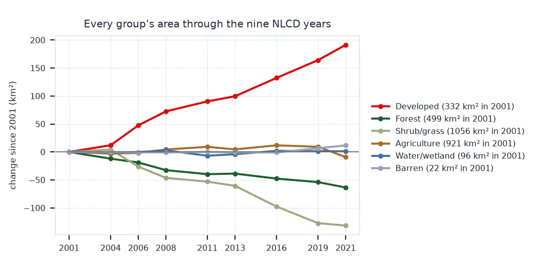
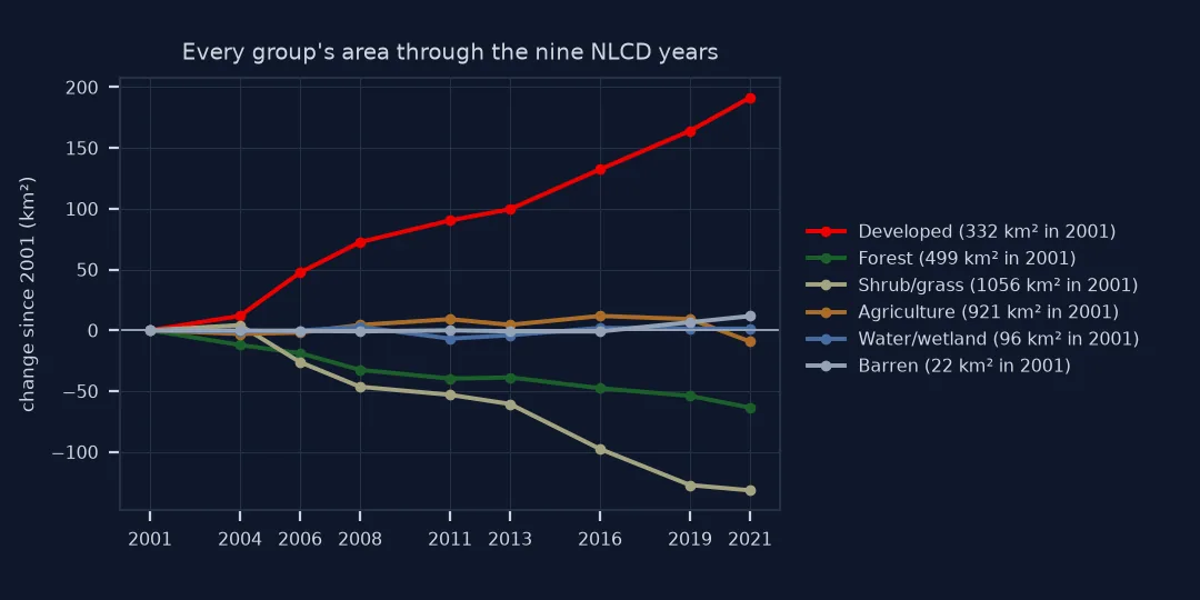
1. Area of every group in every year

areas = pd.DataFrame({y: pd.Series(G[k][valid]).map(GROUP_NAMES).value_counts() * 900 / 1e6 for k, y in enumerate(YEARS)}).T
print(areas.round(0).astype(int).to_string())

      Agriculture  Barren  Developed  Forest  Shrub/grass  Water/wetland
2001          921      22        332     499         1056             96
2004          918      21        344     487         1061             95
2006          919      21        379     480         1030             96
2008          926      21        404     466         1010             99
2011          930      22        422     459         1003             89
2013          926      21        431     460          996             92
2016          933      21        464     451          959             98
2019          930      28        496     445          929             98
2021          912      33        523     435          925             97

Developed land rose in every interval while forest and shrub and grass fell overall. Water and wetland is the one group that goes down and up again, to 89 km² in 2011, a drought year in Texas, and back to 97–99 km² later.

2. When did each pixel last change?

The index of the last year a pixel's group differs from the year before gives its last change:

diff = G[1:] != G[:-1]                                         # True where year k+1 differs from year k
last = np.where(diff.any(axis=0), np.array(YEARS[1:])[diff.shape[0] - 1 - np.argmax(diff[::-1], axis=0)], 0)
lc_years = pd.Series(last[valid & (last > 0)]).value_counts().sort_index()
print((lc_years * 900 / 1e6).round(1).rename("km² last changed in").to_string())

2004    20.9
2006    45.8
2008    35.7
2011    30.5
2013    26.3
2016    57.6
2019    56.0
2021    59.0

Line chart of each group's area relative to 2001 through the nine NLCD years: developed rises steadily to plus 191 square kilometres; shrub and grass falls to about minus 130 and forest to about minus 64; agriculture, water and wetland and barren stay within about 15 square kilometres of where they started. — Each group's path, not just its end points.

3. Separate lasting change from flicker

A pixel that changes and changes back is either a temporary state (a field left fallow, a clearing that regrew) or a classification flip. Count pixels whose 2021 group equals their 2001 group despite changes in between:

back = valid & (changes > 0) & (G[-1] == G[0])
print(f"pixels that changed and ended where they started: {back.sum():,} ({back.sum() / (valid & (changes > 0)).sum():.0%} of pixels that changed at all)")
print("their 2001 group:", pd.Series(G[0][back]).map(GROUP_NAMES).value_counts().head(3).to_dict())

pixels that changed and ended where they started: 40,788 (11% of pixels that changed at all)
their 2001 group: {'Forest': 15653, 'Agriculture': 9182, 'Shrub/grass': 8713}

Forest makes up the largest part of these round trips, about two in five, followed by agriculture and shrub and grass, the classes most easily confused with each other or changed by grazing, fallow and regrowth.

The history of one pixel

The data used on this page

NLCD land cover for all nine years of the 2021 release (2001, 2004, 2006, 2008, 2011, 2013, 2016, 2019, 2021; 30 m) for Williamson County, Texas, from MRLC's WCS, masked to the 2023 Census county outline, and grouped into six classes with a lookup table.

import time
from pathlib import Path

import geopandas as gpd
import numpy as np
import pandas as pd
import rasterio
import rasterio.mask
import requests

Path("data").mkdir(exist_ok=True)
if not Path("data/cb_2023_us_county_20m.zip").exists():
    Path("data/cb_2023_us_county_20m.zip").write_bytes(requests.get("https://www2.census.gov/geo/tiger/GENZ2023/shp/cb_2023_us_county_20m.zip", timeout=300).content)
COUNTY = gpd.read_file("data/cb_2023_us_county_20m.zip").query("GEOID == '48491'").to_crs(5070)
YEARS = [2001, 2004, 2006, 2008, 2011, 2013, 2016, 2019, 2021]
LC = {}
for year in YEARS:
    path = Path(f"data/nlcd_{year}.tif")
    if not path.exists():
        x0, y0, x1, y1 = COUNTY.total_bounds
        for attempt in range(4):
            r = requests.get("https://www.mrlc.gov/geoserver/mrlc_download/wcs", params={"service": "WCS", "version": "2.0.1", "request": "GetCoverage",
                             "coverageId": f"mrlc_download__NLCD_{year}_Land_Cover_L48", "subset": [f"X({x0},{x1})", f"Y({y0},{y1})"], "format": "image/geotiff"}, timeout=300)
            if r.status_code < 500:
                break
            time.sleep(15 * (attempt + 1))
        r.raise_for_status()
        path.write_bytes(r.content)
    with rasterio.open(path) as src:
        LC[year] = rasterio.mask.mask(src, COUNTY.geometry, crop=True, nodata=0)[0][0]
GROUP_NAMES = {1: "Water/wetland", 2: "Developed", 3: "Forest", 4: "Shrub/grass", 5: "Agriculture", 6: "Barren"}
LUT = np.zeros(256, np.uint8)
for codes, g in (((11, 12, 90, 95), 1), ((21, 22, 23, 24), 2), ((41, 42, 43), 3), ((52, 71), 4), ((81, 82), 5), ((31,), 6)):
    LUT[list(codes)] = g
print(f"{len(YEARS)} years, each {LC[2001].shape[1]} x {LC[2001].shape[0]} pixels")

9 years, each 2845 x 1884 pixels

Example 1: the history of one pixel

j, i = np.argwhere(valid & (changes == changes[valid].max()))[0]
print(f"a pixel with {changes[j, i]} changes:", " → ".join(f"{y} {STACK[k, j, i]}" for k, y in enumerate(YEARS)))

a pixel with 8 changes: 2001 41 → 2004 81 → 2006 52 → 2008 41 → 2011 52 → 2013 41 → 2016 11 → 2019 71 → 2021 11

A series is a cube reduced along time

A land cover series is a cube, and most questions about it are reductions along time: the sum of changes, the first or last year something happened, the class in a given year. NumPy's axis arguments do these in one pass over the cube, and a lookup table reclassifies all years at once. Nine years of a county at 30 m fit in about 50 MB as unsigned bytes, so the whole history is in memory; for larger areas, read windows of the stack and process them one at a time.

A land cover history as one array, and the reductions along time.

Consecutive maps from one product series are built to be compared: NLCD detects change and relabels only the changed pixels, so unchanged land keeps its label exactly. Even so, a share of pixels change and change back. Some are real, such as cropland rotating through fallow grass. Others are disagreements between years in classes that are hard to tell apart, such as grassland, pasture and shrub. A history that ends where it started deserves a second look before it is reported as change.

Uneven intervals, memory and permanent development

Time series problems and fixes.

Uneven intervals: NLCD years are two or three years apart; divide by the gap before comparing rates.
Memory: use uint8 for the stack; int64 (NumPy's default for some operations) needs eight times as much.
Developed never reverts in NLCD, so developed pixels have at most one change into developed.
Grouping first: changes between classes of one group (deciduous to evergreen) disappear after grouping; decide which you want to count.
Other series: the same code works for Dynamic World, MapBiomas or annual products, with more noise from pixel-level classification.

Internal links

How to measure urban growth from NLCD — the developed part of this history
How to build a land cover change matrix — two years in detail

FAQ

How do I stack land cover years in Python?

Read each year on the same grid and use np.stack to build a (years, rows, cols) array; compute along axis 0.

How do I count how many times each pixel changed?

Compare consecutive years with stack[1:] != stack[:-1] and sum along the first axis.

How do I find the year a pixel last changed?

Take the comparison array, reverse it along time, find the first True with argmax, and map that index back to the year.

Why do some pixels change and change back?

Some are real temporary states such as fallow fields or regrowth; others are classification differences between years in similar classes.