
Categorical Rasters Explained
On this page
Problem statement
Most raster tools assume the numbers in a grid are quantities: temperatures, elevations, reflectances, which can be averaged, interpolated and smoothed. A land cover raster stores labels that happen to be numbers. The code 42 means evergreen forest; it is not "more" than 41 or "between" 24 and 52. Almost every mistake made with land cover data comes from treating labels as quantities, and almost every useful summary comes from treating them as what they are: categories to be counted.
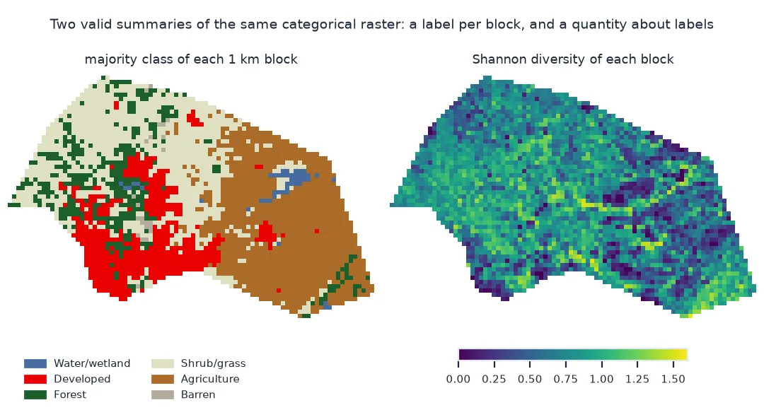
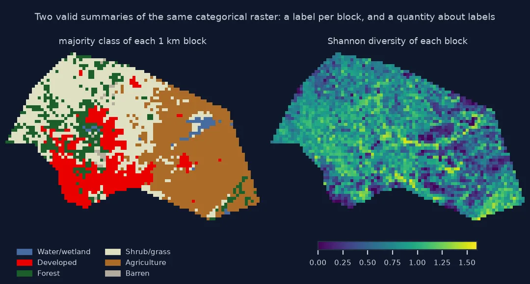
This page sets out what can and cannot be computed from a categorical raster, using NLCD 2021 for Williamson County, Texas: counts and fractions, majority and diversity in blocks, and adjacency, which classes border which.
Quick answer
Every valid summary starts from counts of each class, in an area or a neighbourhood:
blocks = G[:BH * 33, :BW * 33].reshape(BH, 33, BW, 33).transpose(0, 2, 1, 3).reshape(BH, BW, -1)    # 33 x 33 pixels ≈ 1 km
counts = np.stack([(blocks == k).sum(axis=2) for k in GROUP_NAMES], axis=-1)                            # (rows, cols, classes)
valid = counts.sum(axis=2) > 33 * 33 * 0.5
majority = np.array(list(GROUP_NAMES))[counts.argmax(axis=2)]
p = counts / np.maximum(counts.sum(axis=2, keepdims=True), 1)
shannon = -(np.where(p > 0, p * np.log(p), 0)).sum(axis=2)
print(f"{valid.sum():,} blocks of about 1 km²; majority class: {pd.Series(majority[valid]).map(GROUP_NAMES).value_counts().head(3).to_dict()}")
print(f"Shannon diversity: median {np.median(shannon[valid]):.2f}, max {shannon[valid].max():.2f} (ln 6 = {np.log(6):.2f} if all six classes were equal)")
2,987 blocks of about 1 km²; majority class: {'Agriculture': 1059, 'Shrub/grass': 994, 'Developed': 500}
Shannon diversity: median 0.77, max 1.55 (ln 6 = 1.79 if all six classes were equal)
No arithmetic on codes, majority and fractions, adjacency
1. Arithmetic on codes is meaningless
Averaging codes gives numbers between labels; a mean of 50 in a block of grass (71) and developed land (21–24) does not mean shrubland (52):
orig = CODES_ORIG[:BH * 33, :BW * 33].reshape(BH, 33, BW, 33).transpose(0, 2, 1, 3).reshape(BH, BW, -1).astype(float)
orig[orig == 0] = np.nan
code_mean = np.nanmean(orig, axis=2)
near = np.round(code_mean[valid]).astype(int)
in_block = [c in set(b[~np.isnan(b)].astype(int)) for c, b in zip(near, orig[valid])]
print(f"blocks whose mean code rounds to a valid NLCD code: {np.isin(near, list(NLCD_CODES)).mean():.0%}; "
      f"to a class actually present in the block: {np.mean(in_block):.0%}")
blocks whose mean code rounds to a valid NLCD code: 14%; to a class actually present in the block: 11%
In 86% of blocks the mean code is not a land cover code at all, and only 11% land on a class that occurs in the block.
2. Majority and fractions keep the meaning
The majority class is a label, and fractions are quantities about labels; both are valid. They answer different questions, and the majority hides mixtures:
dev_frac = counts[..., list(GROUP_NAMES).index(2)] / np.maximum(counts.sum(axis=2), 1)
mixed = valid & (p.max(axis=2) < 0.5)
print(f"blocks with no class above 50%: {mixed.sum() / valid.sum():.0%}")
print(f"developed land: majority in {(majority[valid] == 2).sum()} blocks, but present in {(dev_frac[valid] > 0).sum()} of {valid.sum()}")
blocks with no class above 50%: 13%
developed land: majority in 500 blocks, but present in 2791 of 2987
3. Adjacency: which classes touch
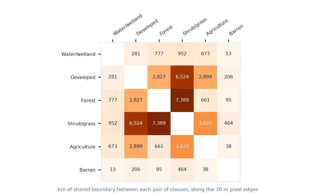
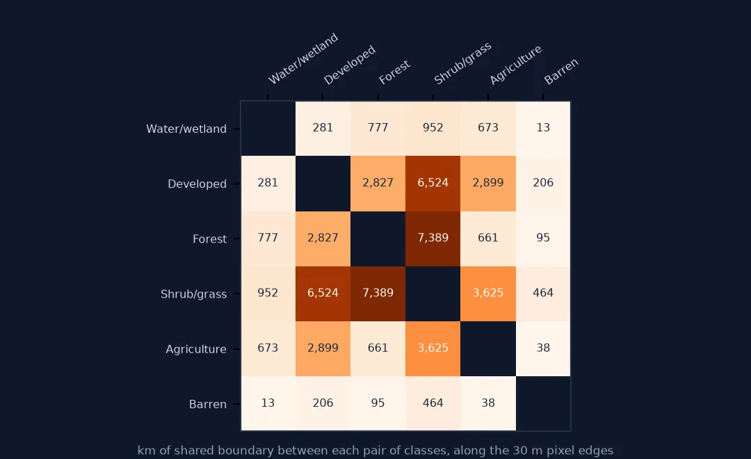
A categorical raster also has a structure that quantities lack: boundaries between classes. Counting neighbouring pairs gives an adjacency matrix, the length of edge shared by each pair of classes:
h = (G[:, :-1], G[:, 1:]); v = (G[:-1, :], G[1:, :])
pairs = pd.concat([pd.DataFrame({"a": a.ravel(), "b": b.ravel()}) for a, b in (h, v)], ignore_index=True)
pairs = pairs[(pairs.a > 0) & (pairs.b > 0) & (pairs.a != pairs.b)]
edge = pd.crosstab(pairs.a.map(GROUP_NAMES), pairs.b.map(GROUP_NAMES)) * 30 / 1000
edge = edge + edge.T                                             # a boundary appears as (a, b) or (b, a); add both
top = edge.where(np.triu(np.ones(edge.shape, bool), 1)).stack().sort_values(ascending=False).head(4)
print({f"{a} | {b}": f"{v:,.0f} km" for (a, b), v in top.items()})
{'Forest | Shrub/grass': '7,389 km', 'Developed | Shrub/grass': '6,524 km', 'Agriculture | Shrub/grass': '3,625 km', 'Agriculture | Developed': '2,899 km'}
Forest meets shrub and grassland along more edge than any other pair, and developed land borders shrub and grass almost as much. On a 30 m grid these lengths follow the pixel staircase and are longer than the real boundaries, but they compare pairs fairly.
The most and least diverse square kilometre
The data used on this page
NLCD 2021 (30 m) for Williamson County, Texas, from MRLC's WCS, masked to the 2023 Census county outline and grouped into six classes with a lookup table.
import time
from pathlib import Path

import geopandas as gpd
import numpy as np
import pandas as pd
import rasterio
import rasterio.mask
import requests

Path("data").mkdir(exist_ok=True)
if not Path("data/cb_2023_us_county_20m.zip").exists():
    Path("data/cb_2023_us_county_20m.zip").write_bytes(requests.get("https://www2.census.gov/geo/tiger/GENZ2023/shp/cb_2023_us_county_20m.zip", timeout=300).content)
COUNTY = gpd.read_file("data/cb_2023_us_county_20m.zip").query("GEOID == '48491'").to_crs(5070)
path = Path("data/nlcd_2021.tif")
if not path.exists():
    x0, y0, x1, y1 = COUNTY.total_bounds
    for attempt in range(4):
        r = requests.get("https://www.mrlc.gov/geoserver/mrlc_download/wcs", params={"service": "WCS", "version": "2.0.1", "request": "GetCoverage",
                         "coverageId": "mrlc_download__NLCD_2021_Land_Cover_L48", "subset": [f"X({x0},{x1})", f"Y({y0},{y1})"], "format": "image/geotiff"}, timeout=300)
        if r.status_code < 500:
            break
        time.sleep(15 * (attempt + 1))
    r.raise_for_status()
    path.write_bytes(r.content)
with rasterio.open(path) as src:
    CODES_ORIG = rasterio.mask.mask(src, COUNTY.geometry, crop=True, nodata=0)[0][0]
NLCD_CODES = {11, 12, 21, 22, 23, 24, 31, 41, 42, 43, 52, 71, 81, 82, 90, 95}
GROUP_NAMES = {1: "Water/wetland", 2: "Developed", 3: "Forest", 4: "Shrub/grass", 5: "Agriculture", 6: "Barren"}
LUT = np.zeros(256, np.uint8)
for codes, g in (((11, 12, 90, 95), 1), ((21, 22, 23, 24), 2), ((41, 42, 43), 3), ((52, 71), 4), ((81, 82), 5), ((31,), 6)):
    LUT[list(codes)] = g
G = LUT[CODES_ORIG]
BH, BW = G.shape[0] // 33, G.shape[1] // 33
print(f"{G.shape[1]} x {G.shape[0]} pixels in {BW} x {BH} blocks of 33 x 33")
2845 x 1884 pixels in 86 x 57 blocks of 33 x 33
Example 1: the most and least diverse square kilometre
for name, idx in (("most diverse", np.nanargmax(np.where(valid, shannon, np.nan))), ("least diverse", np.nanargmin(np.where(valid, shannon, np.nan)))):
    j, i = np.unravel_index(idx, shannon.shape)
    print(f"{name}: H = {abs(shannon[j, i]):.2f};", {GROUP_NAMES[k]: f"{p[j, i, n]:.0%}" for n, k in enumerate(GROUP_NAMES) if p[j, i, n] > 0})
most diverse: H = 1.55; {'Water/wetland': '13%', 'Developed': '12%', 'Forest': '29%', 'Shrub/grass': '19%', 'Agriculture': '27%'}
least diverse: H = 0.00; {'Agriculture': '100%'}
Measurement scales decide the operations
Measurement scales decide which operations make sense. Categorical (nominal) data allow counting, comparing for equality and finding the most common value; nothing else. That rules out means, medians, standard deviations, interpolation, bilinear or cubic resampling, smoothing filters and gradients, all of which treat the numbers as ordered quantities. What remains is still rich: class areas and fractions, majority and diversity in a neighbourhood, transitions between dates, and the geometry of patches and their shared boundaries.
Each of those outputs is either a label (the majority class) or a quantity about labels (a fraction, a count, a length of shared edge), and quantities about labels can be averaged and interpolated like any others. That is the general recipe: turn categories into counts first, then do arithmetic on the counts. Most of the operations on this site's land cover pages are variations on it.
Ordered categories and diversity indices
- Ordered categories: some categorical data are ordinal (burn severity low, moderate, high); medians and ranks are then valid, means still are not.
- Codes in metadata: GeoTIFF colour tables and raster attribute tables (RATs) store class names; keep them with the data.
- Diversity indices: Shannon diversity depends on how many classes exist; compare values only between maps with the same classes.
- Adjacency at 30 m: edge lengths follow the pixel staircase and overstate the length of smooth boundaries.
- Nodata is a category too, and must be excluded from counts, fractions and neighbours.
Internal links
- Why does my resampled land cover have classes that should not be there? — interpolation on codes
- How to summarise land cover by polygon — counts by zone
FAQ
What is a categorical raster?
A raster whose values are labels for categories, such as land cover classes, rather than measured quantities.
Can I average a land cover raster?
No. Average the fractions of each class instead; the mean of class codes has no meaning.
What statistics can I compute on categorical rasters?
Counts, areas and fractions of each class, majority (mode), diversity indices, transition matrices between dates, and patch and adjacency metrics.
How do I aggregate a land cover raster to a coarser grid?
Compute the fraction of each class in every coarse cell; take the majority only if one label per cell is needed.