How to Convert a Land Cover Raster to Polygons in Python

Problem statement

Land cover often needs to leave the raster world: to be overlaid with parcels, edited in a GIS, served as vector tiles or joined to other polygons. Converting a classified raster to polygons is one function call, rasterio.features.shapes, and three decisions made, often unknowingly, along the way. Without removing small patches first, every stray pixel becomes a polygon. With the wrong connectivity, many polygons come out invalid. And simplifying the staircase edges one polygon at a time pulls neighbouring polygons apart, leaving gaps and overlaps.

This page vectorises NLCD 2021 for Williamson County, Texas, grouped into six classes, and measures each decision.

Quick answer

Sieve, polygonise with 4-connectivity, and simplify the polygons together as a coverage:

clean = features.sieve(G, size=25, connectivity=4, mask=G > 0)
polys = gpd.GeoDataFrame(
    [{"group": GROUP_NAMES[int(v)], "geometry": shape(g)} for g, v in features.shapes(clean, mask=clean > 0, transform=TRANSFORM, connectivity=4)],
    crs=5070)
polys["geometry"] = polys.geometry.simplify_coverage(30)
print(f"{len(polys):,} polygons, all valid: {polys.is_valid.all()}; area {polys.area.sum() / 1e6:,.1f} km² "
      f"(raster {np.count_nonzero(G) * 900 / 1e6:,.1f} km²)")
polys.to_file("data/williamson_groups.gpkg", driver="GPKG")

5,563 polygons, all valid: True; area 2,926.1 km² (raster 2,926.2 km²)

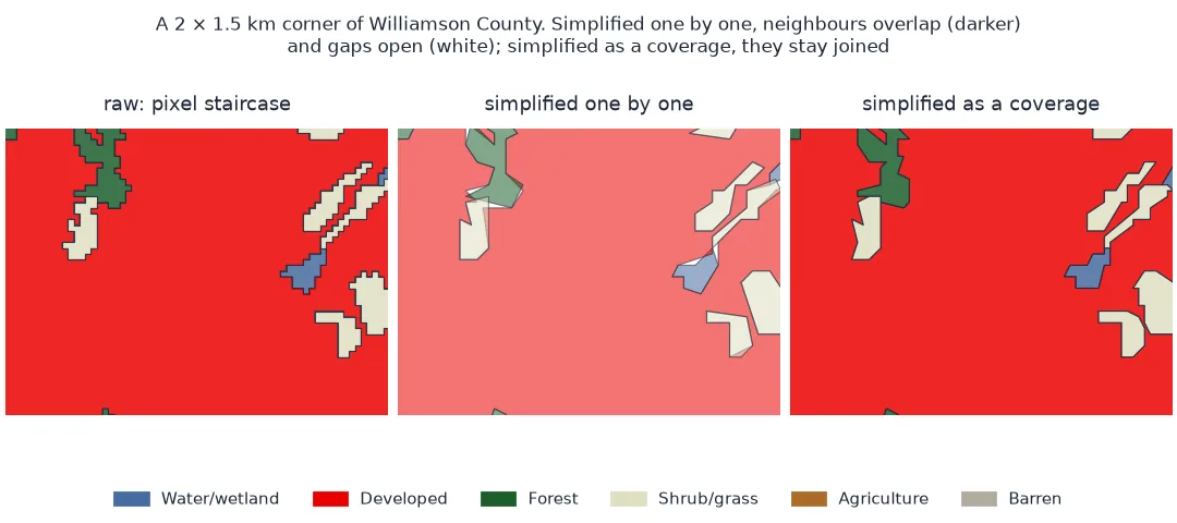
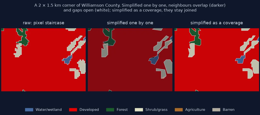
Sieve, use 4-connectivity, simplify the coverage

1. Sieve before polygonising

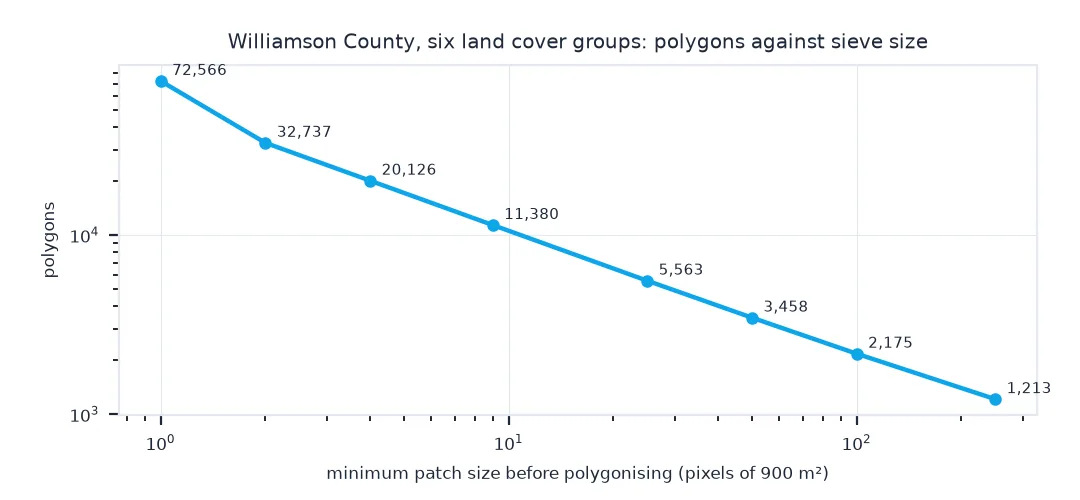
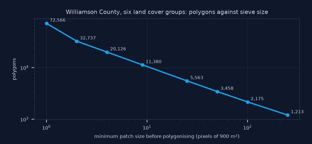
Every connected patch becomes a polygon, including single pixels. A minimum size of 25 pixels (2.25 ha) removes most of them:

for size in (1, 4, 25, 100):
    g = features.sieve(G, size=size, connectivity=4, mask=G > 0) if size > 1 else G
    n = sum(1 for _ in features.shapes(g, mask=g > 0, transform=TRANSFORM, connectivity=4))
    print(f"minimum patch {size:>3} pixels ({size * 0.09:5.2f} ha): {n:>6,} polygons")

minimum patch   1 pixels ( 0.09 ha): 72,566 polygons
minimum patch   4 pixels ( 0.36 ha): 20,126 polygons
minimum patch  25 pixels ( 2.25 ha):  5,563 polygons
minimum patch 100 pixels ( 9.00 ha):  2,175 polygons

2. Use 4-connectivity

With 8-connectivity, pixels that touch only at a corner belong to the same polygon, and its outline passes through that corner twice, which makes the ring self-intersecting:

for conn in (4, 8):
    g = features.sieve(G, size=25, connectivity=conn, mask=G > 0)
    gs = gpd.GeoSeries([shape(geom) for geom, v in features.shapes(g, mask=g > 0, transform=TRANSFORM, connectivity=conn)], crs=5070)
    print(f"{conn}-connectivity: {len(gs):,} polygons, {(~gs.is_valid).mean():.0%} invalid; first reason: {explain_validity(gs[~gs.is_valid].iloc[0]) if (~gs.is_valid).any() else '-'}")

4-connectivity: 5,563 polygons, 0% invalid; first reason: -
8-connectivity: 5,426 polygons, 71% invalid; first reason: Ring Self-intersection[-173775 871185]

3. Simplify the coverage, not the polygons

Raster outlines follow pixel edges, so a 30 m staircase holds many vertices. Simplifying each polygon on its own moves shared edges differently on each side:

raw = gpd.GeoDataFrame([{"geometry": shape(g)} for g, v in features.shapes(clean, mask=clean > 0, transform=TRANSFORM, connectivity=4)], crs=5070)
alone = raw.simplify(30)
together = raw.geometry.simplify_coverage(30)
truth = raw.union_all().area
for name, s in (("one by one", alone), ("as a coverage", together)):
    overlap = s.area.sum() - s.union_all().area
    gaps = truth - s.union_all().area
    print(f"{name:13s}: vertices {s.count_coordinates().sum():,} (from {raw.count_coordinates().sum():,}); overlaps {overlap / 1e6:.1f} km², gaps {gaps / 1e6:.1f} km²")

one by one   : vertices 197,143 (from 664,432); overlaps 23.0 km², gaps 24.3 km²
as a coverage: vertices 340,698 (from 664,432); overlaps 0.0 km², gaps 0.1 km²

Simplifying one by one removes more vertices but opens 24 km² of gaps and piles up 23 km² of overlaps. As a coverage, shared edges stay shared; the 0.1 km² that remains is the county's outer edge, which coverage simplification also smooths unless given simplify_boundary=False.

Polygons per land cover group

The data used on this page

NLCD 2021 (30 m) for Williamson County, Texas, from MRLC's WCS, masked to the 2023 Census county outline and grouped into six classes with a lookup table. Coverage simplification needs Shapely 2.1 (GEOS 3.12) or later and GeoPandas 1.1.

import time
from pathlib import Path

import geopandas as gpd
import numpy as np
import rasterio
import rasterio.mask
import requests
import shapely
from rasterio import features
from shapely.geometry import shape
from shapely.validation import explain_validity

Path("data").mkdir(exist_ok=True)
if not Path("data/cb_2023_us_county_20m.zip").exists():
    Path("data/cb_2023_us_county_20m.zip").write_bytes(requests.get("https://www2.census.gov/geo/tiger/GENZ2023/shp/cb_2023_us_county_20m.zip", timeout=300).content)
COUNTY = gpd.read_file("data/cb_2023_us_county_20m.zip").query("GEOID == '48491'").to_crs(5070)
path = Path("data/nlcd_2021.tif")
if not path.exists():
    x0, y0, x1, y1 = COUNTY.total_bounds
    for attempt in range(4):
        r = requests.get("https://www.mrlc.gov/geoserver/mrlc_download/wcs", params={"service": "WCS", "version": "2.0.1", "request": "GetCoverage",
                         "coverageId": "mrlc_download__NLCD_2021_Land_Cover_L48", "subset": [f"X({x0},{x1})", f"Y({y0},{y1})"], "format": "image/geotiff"}, timeout=300)
        if r.status_code < 500:
            break
        time.sleep(15 * (attempt + 1))
    r.raise_for_status()
    path.write_bytes(r.content)
with rasterio.open(path) as src:
    lc, TRANSFORM = rasterio.mask.mask(src, COUNTY.geometry, crop=True, nodata=0)
GROUP_NAMES = {1: "Water/wetland", 2: "Developed", 3: "Forest", 4: "Shrub/grass", 5: "Agriculture", 6: "Barren"}
LUT = np.zeros(256, np.uint8)
for codes, g in (((11, 12, 90, 95), 1), ((21, 22, 23, 24), 2), ((41, 42, 43), 3), ((52, 71), 4), ((81, 82), 5), ((31,), 6)):
    LUT[list(codes)] = g
G = LUT[lc[0]]
print(f"{G.shape[1]} x {G.shape[0]} pixels; Shapely {shapely.__version__}, GEOS {shapely.geos_version_string}")

2845 x 1884 pixels; Shapely 2.1.2, GEOS 3.13.1

Example 1: polygons per group

summary = polys.assign(km2=polys.area / 1e6).groupby("group").agg(polygons=("km2", "size"), km2=("km2", "sum"), largest=("km2", "max"))
print(summary.round(1).sort_values("km2", ascending=False).to_string())

               polygons    km2  largest
group                                  
Agriculture         977  937.2     22.1
Shrub/grass        2396  890.2     37.4
Developed            60  574.8    569.8
Forest             1599  407.7     11.6
Water/wetland       428   86.7     26.6
Barren              103   29.5      6.5

Developed land is almost one polygon: 569.8 of its 574.8 km² is a single patch, because roads, classed as developed, connect nearly every town and house. Polygon counts of developed land mean little for that reason.

Polygonising is exact

Polygonising traces the boundary of every connected patch of equal values. The result is exact: the polygons' total area equals the pixel count times the pixel area, and their edges are the pixel edges, a staircase of 30 m steps. What makes the output usable is what happens around that step. Sieving decides what counts as a patch. Connectivity decides which pixels belong together, and 4-connectivity keeps every polygon a simple, valid shape. Simplification decides how much of the staircase to keep.

The polygons form a coverage: they tile the area with no gaps or overlaps, and neighbours share their boundaries exactly. Simplifying each polygon independently treats each shared boundary twice, once from each side, and the two simplifications differ, opening slivers of gap and overlap. Coverage simplification, new in GEOS 3.12, simplifies each shared edge once and gives the result to both neighbours, keeping the tiling intact. On older versions, simplify a dissolved boundary network and rebuild polygons from it, or skip simplification.

Holes, large rasters and tolerances

• Holes: patches inside other patches become holes in the surrounding polygon; with 4-connectivity they stay valid.
• Sieve connectivity should match the polygonising connectivity, or patches the sieve kept may split.
• Large rasters: features.shapes streams polygons; for whole states, polygonise tiles and dissolve across tile edges.
• GDAL alternative: gdal_polygonize.py does the same from the command line, with -8 for 8-connectivity.
• Tolerance: a simplification tolerance of about one pixel removes the staircase without moving boundaries more than the data's own resolution.

Internal links

• Why is my land cover change map full of speckle? — sieving as a minimum mapping unit
• Why are my fire perimeter areas wrong? — what invalid polygons do later

FAQ

How do I convert a raster to polygons in Python?

rasterio.features.shapes(array, transform=...) yields one GeoJSON-like geometry and value per connected patch; build a GeoDataFrame from them.

Why are my polygonised raster polygons invalid?

With 8-connectivity, pixels touching at a corner join one polygon whose ring self-intersects at that corner. Use 4-connectivity.

How do I reduce the number of polygons from a raster?

Sieve the raster first (rasterio.features.sieve) to remove patches below a minimum size.

How do I simplify polygons without creating gaps?

Simplify them as a coverage: GeoSeries.simplify_coverage(tolerance) in GeoPandas 1.1, or shapely.coverage_simplify.