
How to Build a Land Cover Change Matrix in Python
On this page
Problem statement
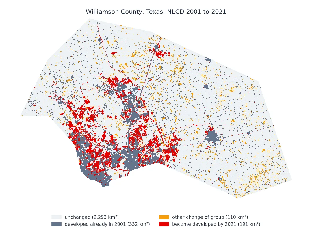
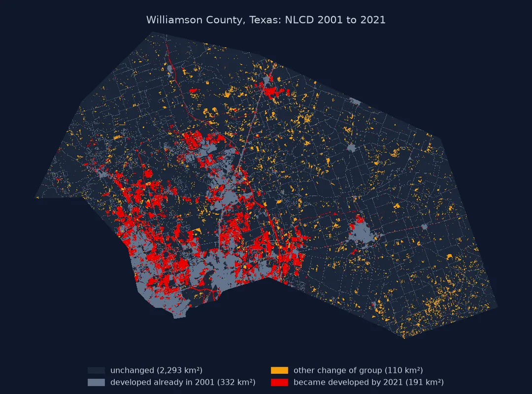
Two land cover maps of the same place, years apart, hold more than two sets of class totals. Comparing totals says that grassland shrank and developed land grew. A change matrix, also called a transition or cross-tabulation matrix, says what became what: how much grassland became houses, how much forest became pasture, and how much stayed put. It separates net change from the gross gains and losses that cancel inside it. It is also where the rules of the product show up: some transitions a map is built never to record.
This page builds the matrix for Williamson County, Texas, between NLCD 2001 and NLCD 2021, at the level of eight broad groups and of all sixteen classes.
Quick answer
Mask both years to the same area, flatten them in the same order, and cross-tabulate. Multiply counts by the pixel area:
valid = (Y2001 > 0) & (Y2021 > 0)
before = pd.Series(Y2001[valid]).map(GROUP).rename("2001")
after = pd.Series(Y2021[valid]).map(GROUP).rename("2021")
matrix = pd.crosstab(before, after) * PIXEL_KM2
print(matrix.round(0).astype(int).to_string())
print(f"changed: {(before != after).mean():.1%} of the county, {(before != after).sum() * PIXEL_KM2:,.0f} km²")
2021 Agriculture Barren Developed Forest Grassland Shrub Water Wetland
2001
Agriculture 877 1 18 2 8 15 0 0
Barren 0 19 1 0 1 0 0 0
Developed 0 0 332 0 0 0 0 0
Forest 1 3 51 426 10 7 0 0
Grassland 31 9 109 2 737 4 2 0
Shrub 3 1 11 5 1 141 0 0
Water 0 0 0 0 0 0 29 1
Wetland 0 0 1 0 0 0 0 64
changed: 10.3% of the county, 301 km²
Gross against net, ranked transitions, the product's rules
1. Separate gross from net
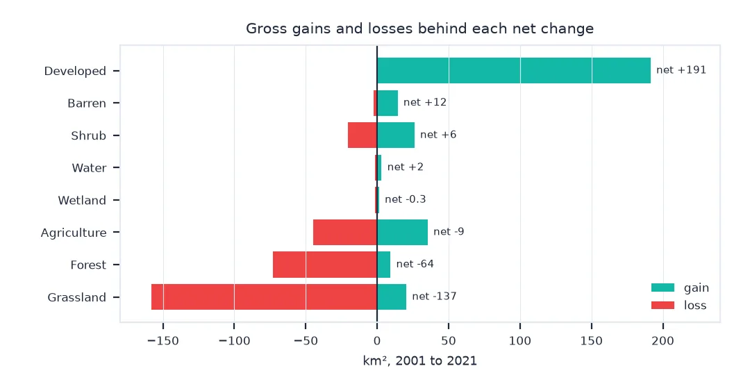
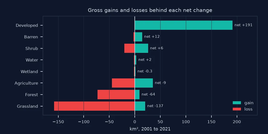
The diagonal is persistence. A row's off-diagonal cells are that class's losses; a column's are its gains:
persist = pd.Series(np.diag(matrix), index=matrix.index)
summary = pd.DataFrame({"2001": matrix.sum(axis=1), "2021": matrix.sum(axis=0),
                        "gain": matrix.sum(axis=0) - persist, "loss": matrix.sum(axis=1) - persist})
summary["net"] = summary.gain - summary.loss
summary["swap"] = 2 * np.minimum(summary.gain, summary.loss)          # change that cancels out
print(summary.round(1).sort_values("net").to_string())
2001 2021 gain loss net swap
Grassland 895.2 757.8 20.4 157.8 -137.4 40.9
Forest 499.0 435.5 9.3 72.9 -63.5 18.7
Agriculture 921.1 912.0 35.4 44.5 -9.2 70.8
Wetland 65.4 65.1 1.4 1.6 -0.3 2.7
Water 30.9 32.4 3.1 1.6 1.5 3.2
Shrub 161.3 167.0 26.1 20.4 5.7 40.7
Barren 21.6 33.3 14.4 2.7 11.7 5.3
Developed 331.8 523.2 191.4 0.0 191.4 0.0
Grassland and forest show the largest net losses and developed land the largest net gain. Agriculture's small net change hides gains and losses of tens of square kilometres each, swapping location rather than shrinking.
2. Rank the transitions
pairs = matrix.stack()
pairs = pairs[[a != b for a, b in pairs.index]].sort_values(ascending=False)
print(pairs.head(6).round(1).to_string())
print(f"top transition's share of all change: {pairs.iloc[0] / pairs.sum():.0%}")
2001 2021
Grassland Developed 109.1
Forest Developed 51.3
Grassland Agriculture 31.2
Agriculture Developed 17.9
Shrub 14.5
Shrub Developed 10.7
top transition's share of all change: 36%
3. Look inside the groups
Grouping hides change between classes of the same group. Developed land has four intensity classes, and land that was already developed can still intensify:
full = pd.crosstab(pd.Series(Y2001[valid], name="2001"), pd.Series(Y2021[valid], name="2021")) * PIXEL_KM2
dev = [21, 22, 23, 24]
within = full.loc[dev, dev].to_numpy().sum() - np.trace(full.loc[dev, dev].to_numpy())
print(f"change within developed classes: {within:.1f} km² (invisible in the grouped matrix)")
print(full.loc[dev, dev].round(1).to_string())
change within developed classes: 28.9 km² (invisible in the grouped matrix)
2021 21 22 23 24
2001
21 133.0 5.2 14.2 2.6
22 0.0 80.0 3.7 2.8
23 0.0 0.0 67.9 0.4
24 0.0 0.0 0.0 21.9
4. Check the product's rules
In the grouped matrix, developed land lost almost nothing:
lost = matrix.loc["Developed"].drop("Developed").sum()
print(f"developed in 2001, not developed in 2021: {lost:.2f} km², {lost / PIXEL_KM2:.0f} pixels of {valid.sum():,}")
down = np.tril(full.loc[dev, dev].to_numpy(), -1).sum()        # rows are 2001: below the diagonal = lower intensity in 2021
print(f"developed pixels that moved to a lower intensity: {down:.2f} km²")
developed in 2001, not developed in 2021: 0.01 km², 8 pixels of 3,251,319
developed pixels that moved to a lower intensity: 0.00 km²
That is a rule of NLCD's change detection, not a fact about Williamson County: once developed, a pixel stays developed (8 pixels in 3.25 million are the exception) and never moves to a lower intensity. Demolitions and redevelopment to parkland exist but are not mapped. Every product has rules like this, and a change matrix is where to find them.
Where each 2001 class went
The data used on this page
NLCD 2001 and 2021 (2021 release, 30 m) for Williamson County, Texas, from MRLC's WCS (see how to download NLCD), masked with the 2023 Census county outline. Both years share the same grid, so pixels correspond one to one.
import time
from pathlib import Path

import geopandas as gpd
import numpy as np
import pandas as pd
import rasterio
import rasterio.mask
import requests

Path("data").mkdir(exist_ok=True)
WCS = "https://www.mrlc.gov/geoserver/mrlc_download/wcs"
if not Path("data/cb_2023_us_county_20m.zip").exists():
    Path("data/cb_2023_us_county_20m.zip").write_bytes(requests.get("https://www2.census.gov/geo/tiger/GENZ2023/shp/cb_2023_us_county_20m.zip", timeout=300).content)
COUNTY = gpd.read_file("data/cb_2023_us_county_20m.zip").query("GEOID == '48491'").to_crs(5070)


def nlcd(year):
    path = Path(f"data/nlcd_{year}.tif")
    if not path.exists():
        x0, y0, x1, y1 = COUNTY.total_bounds
        for attempt in range(4):
            r = requests.get(WCS, params={"service": "WCS", "version": "2.0.1", "request": "GetCoverage",
                                          "coverageId": f"mrlc_download__NLCD_{year}_Land_Cover_L48",
                                          "subset": [f"X({x0},{x1})", f"Y({y0},{y1})"], "format": "image/geotiff"}, timeout=300)
            if r.status_code < 500:
                break
            time.sleep(15 * (attempt + 1))
        r.raise_for_status()
        path.write_bytes(r.content)
    with rasterio.open(path) as src:
        a, tr = rasterio.mask.mask(src, COUNTY.geometry, crop=True, nodata=0)
    return a[0], tr


Y2001, TRANSFORM = nlcd(2001)
Y2021, _ = nlcd(2021)
PIXEL_KM2 = 30 * 30 / 1e6
GROUP = {11: "Water", 21: "Developed", 22: "Developed", 23: "Developed", 24: "Developed", 31: "Barren",
         41: "Forest", 42: "Forest", 43: "Forest", 52: "Shrub", 71: "Grassland", 81: "Agriculture", 82: "Agriculture",
         90: "Wetland", 95: "Wetland"}
print(f"grids {Y2001.shape} and {Y2021.shape}, same transform: {TRANSFORM.almost_equals(_)}")
grids (1884, 2845) and (1884, 2845), same transform: True
Example 1: where each 2001 class went, in per cent
rows = matrix.div(matrix.sum(axis=1), axis=0) * 100
print(rows.loc[["Grassland", "Forest", "Agriculture"], ["Developed", "Grassland", "Forest", "Agriculture", "Shrub"]].round(1).to_string())
2021 Developed Grassland Forest Agriculture Shrub
2001
Grassland 12.2 82.4 0.2 3.5 0.5
Forest 10.3 2.0 85.4 0.2 1.4
Agriculture 1.9 0.9 0.2 95.2 1.6
The categorical version of subtracting two rasters
A change matrix is the categorical version of subtracting two rasters. Subtraction is meaningless for class codes (82 minus 71 is not a land cover), so instead each pixel's pair of classes is counted. Row totals are the first map, column totals the second, the diagonal is what stayed, and every off-diagonal cell is one kind of change with its area. Gains, losses, net change and swap all come from those sums. Swap is the part of a class's change that cancels out: land gained in one place and lost in another.
Two cautions apply to any matrix. Map errors appear as change: two classifications of an unchanged pixel can disagree, and those disagreements add up to change that never happened. Products built for change, like NLCD's consistent series, reduce this by detecting change first and relabelling only changed pixels, and they encode rules such as "developed never reverts". Comparing two unrelated products cell by cell gives a matrix full of differences in definition and method.
Same grid, masks and grouping
- Same grid: both maps must share the grid; reprojecting one with anything but nearest neighbour invents classes.
- Masks: use the same mask for both years, and drop pixels that are nodata in either.
- Area: multiply counts by the true pixel area; in a geographic CRS that varies with latitude.
- Grouping: decide the groups before looking at the results, and report change within groups if it matters.
- Small changes: single-pixel changes are often noise; a minimum mapping unit or a majority filter removes speckle before counting.
Internal links
- How to download NLCD land cover — the data used here
- Land cover products explained — why products differ
FAQ
What is a land cover change matrix?
A cross-tabulation of two land cover maps of the same area: rows are classes in the first year, columns in the second, and each cell the area that went from one to the other.
How do I make a transition matrix from two rasters in Python?
Read both rasters on the same grid, mask nodata, flatten them, and use pd.crosstab; multiply the counts by the pixel area.
What is the difference between net and gross change?
Net change is the difference between a class's totals; gross change is its gains plus its losses. A class can change a lot gross with almost no net change.
Why does NLCD show no loss of developed land?
The NLCD change methodology does not allow developed pixels to revert to other classes or to lower intensity. It is a rule of the product.