How to Make an Interactive Map With GeoPandas explore()

Problem statement

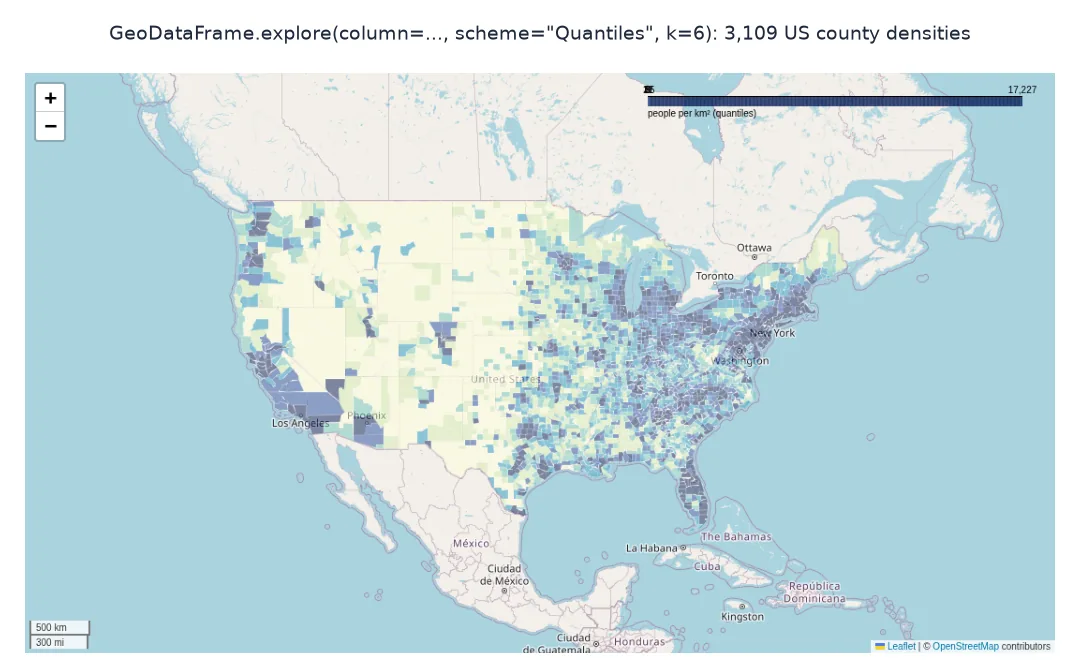
GeoDataFrame.explore() turns any GeoDataFrame into an interactive Leaflet map in one line: hover tooltips, a basemap, a legend and classification all come from the data. It is the quickest way to look at spatial data in a notebook and a good start for a shareable HTML map, but its many keyword arguments decide whether the result is readable: how values are classified, which columns appear on hover, how layers are combined, and how large the file becomes.

This page maps the 2023 population density of US counties with explore(), compares classification schemes from mapclassify, adds a second layer of airports to the same map, controls tooltips and popups, and checks what happens with date columns that plain Folium cannot serialise.

Quick answer

Pass the column to colour by and a classification scheme; explore() returns a Folium map:

m = G.explore(column="density_km2", scheme="Quantiles", k=6, cmap="YlGnBu",
              tooltip=["NAME", "density_txt", "pop_txt"], tooltip_kwds={"aliases": ["County", "People per km²", "Population"]},
              legend_kwds={"caption": "people per km² (quantiles)"}, style_kwds={"weight": 0.2, "color": "white"})
m.save("data/explore_density.html")
print(f"{type(m).__module__}.{type(m).__name__}; HTML {Path('data/explore_density.html').stat().st_size / 1e6:.2f} MB")

folium.folium.Map; HTML 2.99 MB

explore() returns an ordinary folium.Map, here saved as a 2.99 MB page with six quantile classes, a legend and three tooltip fields.

Classification schemes, a second layer, tooltips and size

1. Classification schemes

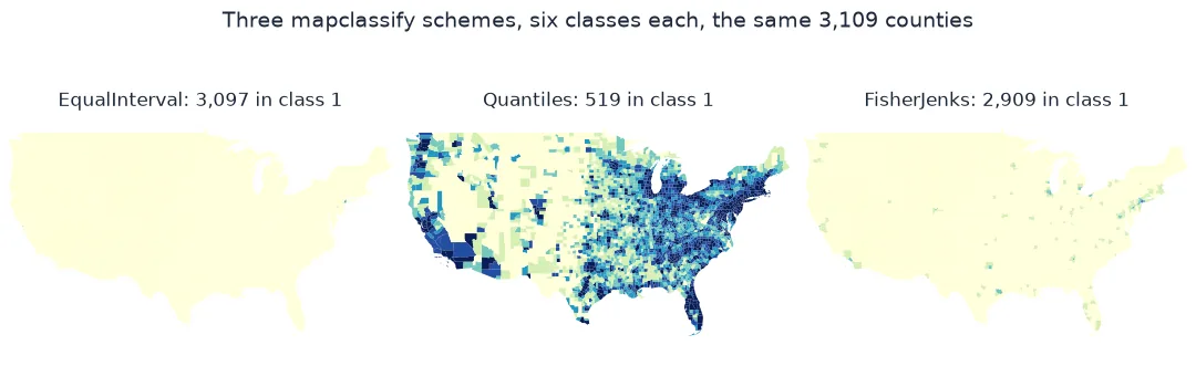
scheme takes any mapclassify classifier by name. Compare how three of them split the 3,109 counties into six classes:

import mapclassify
for name in ("EqualInterval", "Quantiles", "FisherJenks"):
    c = getattr(mapclassify, name)(G.density_km2, k=6)
    print(f"{name:>13}: upper bounds {', '.join(f'{b:,.0f}' for b in c.bins)}; counts {c.counts.tolist()}")

EqualInterval: upper bounds 2,871, 5,742, 8,613, 11,484, 14,356, 17,227; counts [3097, 7, 2, 2, 0, 1]
    Quantiles: upper bounds 3, 9, 17, 31, 85, 17,227; counts [519, 518, 518, 518, 518, 518]
  FisherJenks: upper bounds 269, 985, 2,434, 5,141, 9,667, 17,227; counts [2909, 156, 31, 8, 4, 1]

Equal intervals put 3,097 of the 3,109 counties in the first class, below 2,871 people per km². Quantiles put 518 or 519 counties in each class, with breaks at 3, 9, 17, 31 and 85 people per km². Fisher-Jenks, which minimises the variance within classes, isolates the extremes: 2,909 counties fall below 269, and Manhattan has a class of its own.

2. Add a second layer

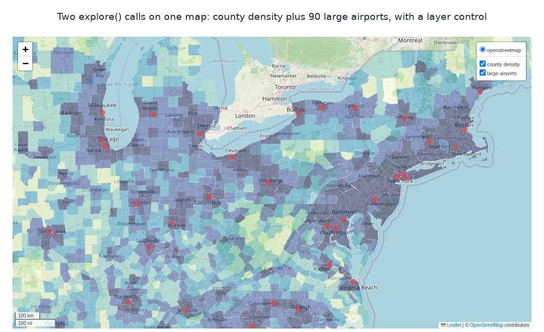
Pass the existing map as m= to draw another GeoDataFrame on top, and add a layer control to switch them:

import folium
m2 = G.explore(column="density_km2", scheme="Quantiles", k=6, cmap="YlGnBu", name="county density", tooltip=["NAME", "density_txt"],
               style_kwds={"weight": 0.2, "color": "white"}, legend=False)
AP.explore(m=m2, color="#ef4444", name="large airports", tooltip=["name", "iata_code"], marker_kwds={"radius": 4})
folium.LayerControl().add_to(m2)
m2.save("data/explore_layers.html")
print(f"layers: {sum(isinstance(c, folium.GeoJson) for c in m2._children.values())} GeoJSON; airports {len(AP)}; HTML {Path('data/explore_layers.html').stat().st_size / 1e6:.2f} MB")

layers: 2 GeoJSON; airports 90; HTML 3.04 MB

The map holds two GeoJSON layers, the counties and the 90 airports, with a control to toggle them. The airports add only 0.05 MB.

3. Tooltips, popups and file size

tooltip= only decides what is shown on hover. explore() writes every column of the GeoDataFrame into the page either way, so to make the file smaller, select the columns before calling it:

five = ["NAME", "density_km2", "density_txt", "pop_txt", "geometry"]
for label, gdf, kw in (("all columns, tooltip with every column", G, {}),
                       ("all columns, three tooltip columns", G, {"tooltip": ["NAME", "density_txt", "pop_txt"]}),
                       ("all columns, no tooltip", G, {"tooltip": False}),
                       ("five columns selected first", G[five], {"tooltip": ["NAME", "density_txt", "pop_txt"]})):
    gdf.explore(column="density_km2", scheme="Quantiles", k=6, **kw).save("data/explore_size.html")
    print(f"{label:>38}: {Path('data/explore_size.html').stat().st_size / 1e6:.2f} MB")
print(f"columns in G: {len(G.columns)}")

all columns, tooltip with every column: 2.99 MB
    all columns, three tooltip columns: 2.99 MB
               all columns, no tooltip: 2.99 MB
           five columns selected first: 2.02 MB
columns in G: 19

With all 19 columns in the GeoDataFrame, the file is 2.99 MB whether the tooltip shows every column, three of them or none, because explore() writes every column into the page either way. Selecting five columns first brings it down to 2.02 MB.

Date columns in explore()

The data used on this page

The US Census Bureau's 2023 county cartographic boundaries (1:20 million) and Vintage 2023 county population estimates, with areas measured in EPSG:5070, and the large US airports from OurAirports. explore() needs folium, matplotlib and, for scheme, mapclassify.

from pathlib import Path

import geopandas as gpd
import pandas as pd
import requests

Path("data").mkdir(exist_ok=True)
def cached(path, url):
    p = Path(path)
    if not p.exists():
        r = requests.get(url, timeout=600)
        r.raise_for_status()
        p.write_bytes(r.content)
    return p
C = gpd.read_file(cached("data/cb_2023_us_county_20m.zip", "https://www2.census.gov/geo/tiger/GENZ2023/shp/cb_2023_us_county_20m.zip")).to_crs(4326)
est = pd.read_csv(cached("data/co-est2023-alldata.csv", "https://www2.census.gov/programs-surveys/popest/datasets/2020-2023/counties/totals/co-est2023-alldata.csv"),
                  encoding="latin-1", dtype={"STATE": str, "COUNTY": str})
est = est[est.SUMLEV == 50].assign(GEOID=lambda d: d.STATE + d.COUNTY)[["GEOID", "STNAME", "CTYNAME", "POPESTIMATE2023"]]
G = C[~C.STATEFP.isin(["02", "15", "72"])].merge(est, on="GEOID")
G["density_km2"] = G.POPESTIMATE2023 / (G.to_crs(5070).area / 1e6)
G["NAME"] = G.CTYNAME + ", " + G.STNAME
G["density_txt"] = G.density_km2.map("{:,.1f}".format)
G["pop_txt"] = G.POPESTIMATE2023.map("{:,}".format)
G["geometry"] = G.geometry.simplify(0.01, preserve_topology=True)
A = pd.read_csv(cached("data/airports.csv", "https://davidmegginson.github.io/ourairports-data/airports.csv"), keep_default_na=False, na_values=[""])
A = A[(A.iso_country == "US") & (A.type == "large_airport") & A.longitude_deg.between(-130, -60)]
AP = gpd.GeoDataFrame(A, geometry=gpd.points_from_xy(A.longitude_deg, A.latitude_deg), crs=4326)
print(f"{len(G):,} counties; {len(AP)} large airports in the conterminous US")

3,109 counties; 90 large airports in the conterminous US

The data covers 3,109 counties, plus the 90 large airports of the conterminous US for the second layer.

Example 1: date columns

Folium's GeoJson fails on pandas Timestamp values. Add a date column and compare:

G["estimated"] = pd.Timestamp("2023-07-01")
try:
    folium.GeoJson(G[["NAME", "estimated", "geometry"]]).add_to(folium.Map())
    print("folium.GeoJson: ok")
except TypeError as e:
    print(f"folium.GeoJson: TypeError: {e}")
m3 = G[["NAME", "estimated", "geometry"]].explore(tooltip=["NAME", "estimated"])
print(f"explore(): ok; the date in the page: {'2023-07-01' in m3.get_root().render()}")
G = G.drop(columns="estimated")

folium.GeoJson: TypeError: Object of type Timestamp is not JSON serializable
explore(): ok; the date in the page: True

Plain Folium raises TypeError: Object of type Timestamp is not JSON serializable. explore() converts the dates to strings and the page shows 2023-07-01.

GeoPandas' wrapper around Folium

explore() is GeoPandas' wrapper around Folium. It converts the GeoDataFrame to EPSG:4326 if needed, writes it as a GeoJSON layer, styles each feature from the column through a matplotlib colormap, classifies numeric values with mapclassify when scheme is given, adds a legend and tooltips, and returns the folium.Map, which can then be extended with anything Folium offers or passed back in with m= for the next layer. Without scheme, values map continuously onto the colormap, which on skewed data like population density makes nearly everything one colour.

The file is the GeoJSON plus the page around it, so its size comes from the geometry and from every column of the GeoDataFrame, whether or not a tooltip shows it. Simplifying the geometry and selecting the columns before calling explore() keeps a national county map light enough to share, and explore() also takes care of details such as converting dates to strings that plain Folium leaves to you.

Categorical columns, missing values and tiles

• Categorical columns: string columns get a categorical colormap and legend automatically; pass categorical=True for integer codes.
• Missing values: missing_kwds={"color": "lightgrey"} gives NaN features their own style.
• Tiles: tiles= takes any Folium tile name or an xyzservices provider; CARTO's raster tiles now return an "API KEY REQUIRED" tile, so keep the OpenStreetMap default or use a provider you have access to.
• Points: marker_type="circle_marker" (the default for points) scales with zoom in pixels; "circle" uses a radius in metres.

Internal links

• How to make a Folium choropleth with tooltips in Python — the same map in plain Folium
• Choropleth classification explained — the schemes behind scheme=
• Fixing Folium Timestamp is not JSON serializable — the error explore() avoids

FAQ

How do I make an interactive map from a GeoDataFrame?

Call gdf.explore(); it returns a Folium map that displays in Jupyter or can be saved with .save("map.html").

How do I change the classification in explore()?

Pass scheme="Quantiles" (or any mapclassify classifier name) and k for the number of classes; mapclassify must be installed.

How do I plot two GeoDataFrames on one explore() map?

Call explore() on the second with m= set to the map returned by the first.

How do I choose which columns show on hover?

Pass a list of column names as tooltip, and tooltip_kwds={"aliases": [...]} to rename them.