How to Map a Million Points With Lonboard in Python

Problem statement

Folium and Plotly slow down long before a million points: the data is written into the page as text, then parsed and drawn by the browser one marker at a time. Lonboard, from Development Seed, takes a different path: it moves a GeoDataFrame to the browser as binary GeoArrow data and draws it with deck.gl on the GPU, so a million points pan and zoom smoothly in a notebook or a saved HTML page.

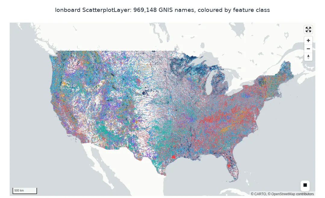
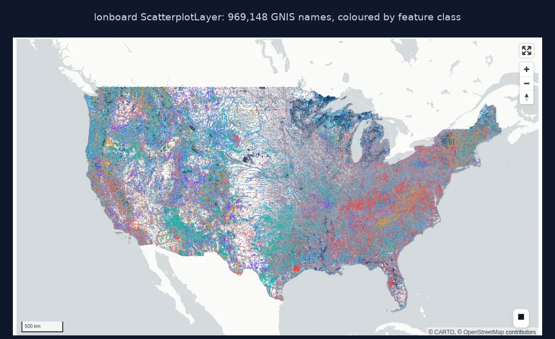
This page maps every one of the roughly one million named places in the US Geological Survey's Geographic Names Information System (GNIS) with lonboard: a one-line viz(), a ScatterplotLayer coloured by feature class, the file size compared with a Folium page of the same points, and the effect of keeping only the columns that are needed.

Quick answer

Pass a GeoDataFrame to viz() and save the map:

from lonboard import viz
m = viz(P[["feature_name", "feature_class", "geometry"]])
m.to_html("data/gnis_viz.html")
print(f"points: {len(P):,}; HTML {Path('data/gnis_viz.html').stat().st_size / 1e6:.1f} MB ({Path('data/gnis_viz.html').stat().st_size / len(P):.0f} bytes per point)")

points: 969,148; HTML 33.2 MB (34 bytes per point)

All 969,148 points, with their names and classes, go into a 33.2 MB page, 34 bytes per point.

Colour by category, compare with Folium, send few columns

1. Colour by category

Build a ScatterplotLayer and give it an array of colours, one row per point. apply_categorical_cmap maps the class names to RGB values:

from lonboard import Map, ScatterplotLayer
from lonboard.colormap import apply_categorical_cmap
top = P.feature_class.value_counts().index[:6]
P["cls"] = P.feature_class.where(P.feature_class.isin(top), "Other")
cmap = dict(zip(list(top) + ["Other"], [(14, 165, 233), (239, 68, 68), (20, 184, 166), (26, 58, 107), (245, 158, 11), (124, 58, 237), (148, 163, 184)]))
layer = ScatterplotLayer.from_geopandas(P[["feature_name", "cls", "geometry"]], get_fill_color=apply_categorical_cmap(P.cls, cmap),
                                        radius_min_pixels=0.6, radius_max_pixels=4, opacity=0.6, pickable=True)
Map(layer, view_state={"longitude": -98, "latitude": 39, "zoom": 3.4}).to_html("data/gnis_classes.html")
print(P.cls.value_counts().to_string())

cls
Other              271719
Stream             230963
Populated Place    185319
Reservoir           72950
Lake                70126
Summit              69252
Valley              68819

The six most common classes are streams (230,963), populated places (185,319), reservoirs, lakes, summits and valleys. The remaining 271,719 names, in dozens of other classes, share one grey.

2. Compared with Folium

Write the same points as a Folium FastMarkerCluster page, which stores only the coordinates, then open both pages in headless Chromium and read how much JavaScript memory each needs once the map is drawn:

import folium, functools, http.server, socketserver, threading
from folium.plugins import FastMarkerCluster
from playwright.sync_api import sync_playwright
fm = folium.Map(location=[39, -98], zoom_start=4)
FastMarkerCluster(np.c_[P.geometry.y, P.geometry.x].tolist()).add_to(fm)
fm.save("data/gnis_folium.html")

class Quiet(http.server.SimpleHTTPRequestHandler):
    def log_message(self, *a): pass
srv = socketserver.TCPServer(("127.0.0.1", 0), functools.partial(Quiet, directory="data"))
threading.Thread(target=srv.serve_forever, daemon=True).start()
heap = {}
with sync_playwright() as pw:
    browser = pw.chromium.launch()
    for f, drawn in (("gnis_viz.html", "canvas"), ("gnis_folium.html", ".marker-cluster")):
        page = browser.new_page(viewport={"width": 1000, "height": 600})
        page.goto(f"http://127.0.0.1:{srv.server_address[1]}/{f}", timeout=300000)
        page.wait_for_selector(drawn, timeout=300000); page.wait_for_timeout(3000)
        heap[f] = page.evaluate("performance.memory.usedJSHeapSize") / 1e6
        page.close()
    browser.close()
srv.shutdown()
for f in heap:
    print(f"{f:>16}: file {Path('data/' + f).stat().st_size / 1e6:5.1f} MB")
print(f"lonboard page under 500 MB of JavaScript memory: {heap['gnis_viz.html'] < 500}")
print(f"Folium page over 1 GB of JavaScript memory: {heap['gnis_folium.html'] > 1000}")

   gnis_viz.html: file  33.2 MB
gnis_folium.html: file  26.2 MB
lonboard page under 500 MB of JavaScript memory: True
Folium page over 1 GB of JavaScript memory: True

The files are of similar size: 26.2 MB for Folium's coordinates against 33.2 MB for lonboard with names and classes. The difference is in the browser. Once drawn, the lonboard page needed less than 500 MB of JavaScript memory, while the Folium page needed more than a gigabyte, because its clustering plugin creates a JavaScript object for each of the 969,148 markers.

3. Send only the columns you need

Every column passed to lonboard goes into the page. Compare all 21 GNIS columns with the geometry alone:

viz(P.drop(columns="cls")).to_html("data/gnis_all_columns.html")
viz(P[["geometry"]]).to_html("data/gnis_geometry_only.html")
for f in ("gnis_all_columns.html", "gnis_viz.html", "gnis_geometry_only.html"):
    print(f"{f:>23}: {Path('data/' + f).stat().st_size / 1e6:6.1f} MB")

  gnis_all_columns.html:   87.7 MB
          gnis_viz.html:   33.2 MB
gnis_geometry_only.html:   23.6 MB

Passing all 21 GNIS columns makes an 87.7 MB page. The two columns the map uses keep it at 33.2 MB, and the geometry alone at 23.6 MB.

The rows that were dropped

The data used on this page

The national file of the GNIS Domestic Names dataset, the US federal standard for geographic names, published by the USGS as a pipe-separated text file. Rows with missing or impossible coordinates are dropped. Lonboard 0.17 is used, with GeoPandas and pyarrow.

import zipfile
from pathlib import Path

import geopandas as gpd
import numpy as np
import pandas as pd
import requests

Path("data").mkdir(exist_ok=True)
p = Path("data/DomesticNames_National_Text.zip")
if not p.exists():
    r = requests.get("https://prd-tnm.s3.amazonaws.com/StagedProducts/GeographicNames/DomesticNames/DomesticNames_National_Text.zip", timeout=900)
    r.raise_for_status()
    p.write_bytes(r.content)
with zipfile.ZipFile(p) as z:
    N = pd.read_csv(z.open("Text/DomesticNames_National.txt"), sep="|", low_memory=False)
ok = N.prim_lat_dec.between(-90, 90) & N.prim_long_dec.between(-180, 180) & ~((N.prim_lat_dec == 0) & (N.prim_long_dec == 0))
P = gpd.GeoDataFrame(N[ok], geometry=gpd.points_from_xy(N.prim_long_dec[ok], N.prim_lat_dec[ok]), crs=4326).reset_index(drop=True)
print(f"GNIS rows: {len(N):,}; kept {len(P):,}; dropped {(~ok).sum():,} with missing or impossible coordinates")

GNIS rows: 981,708; kept 969,148; dropped 12,560 with missing or impossible coordinates

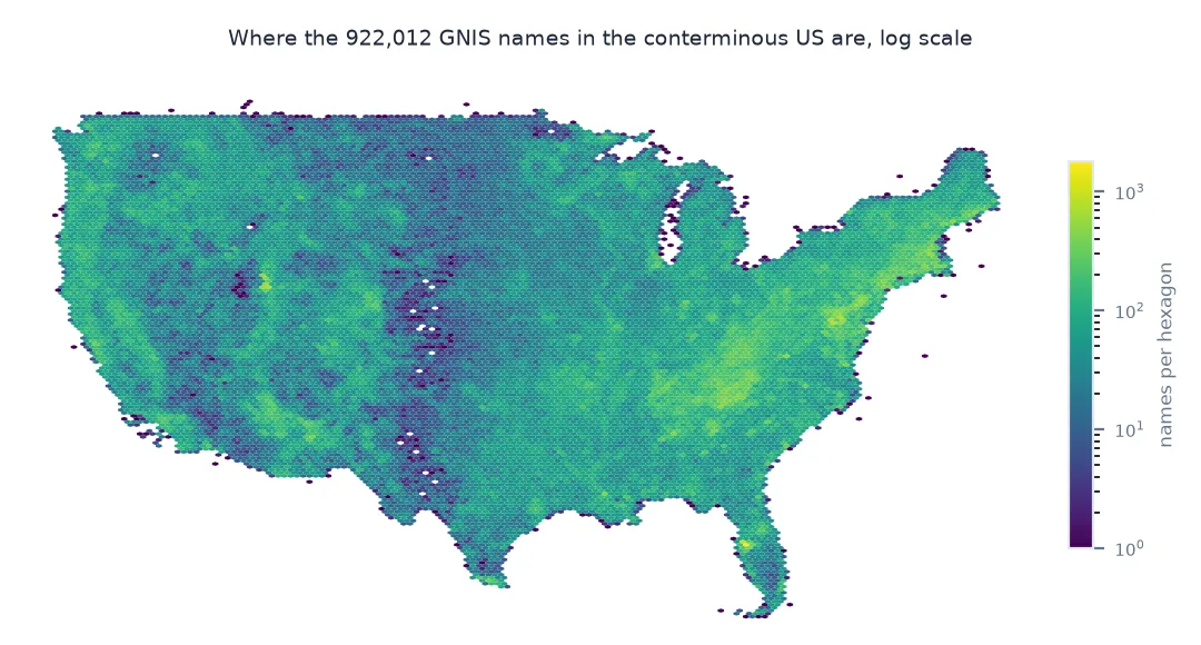
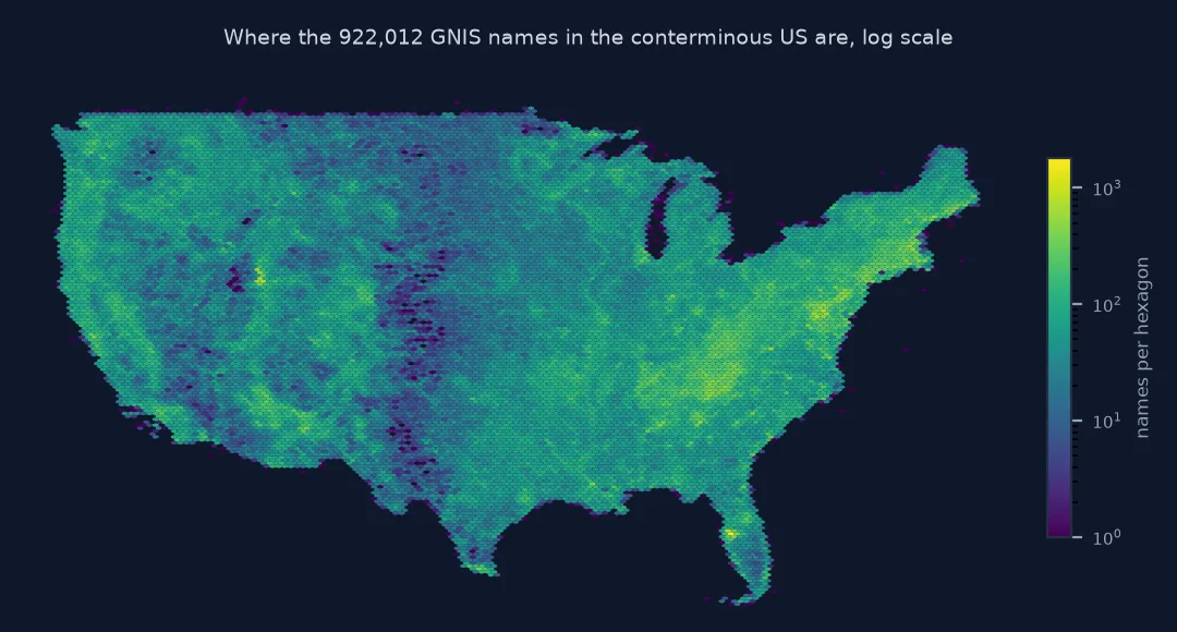
The national file has 981,708 names. 969,148 of them have usable coordinates, and 12,560 are dropped.

Example 1: the rows that were dropped

Check what the coordinate filter removed before trusting the map:

bad = N[~ok]
print(f"longitude below -180: {(bad.prim_long_dec < -180).sum()}; at 0, 0: {((bad.prim_lat_dec == 0) & (bad.prim_long_dec == 0)).sum():,}")
print(bad.feature_class.value_counts().head(4).to_string())

longitude below -180: 3; at 0, 0: 12,557
feature_class
Populated Place    5603
Spring             2476
Stream             1624
Summit              460

Almost all the dropped rows, 12,557, have coordinates of exactly 0, 0, GNIS's placeholder for an unknown location. Three have longitudes below −180. Most are populated places, springs and streams.

GeoArrow instead of GeoJSON text

Lonboard is a Jupyter widget built on anywidget and deck.gl. Instead of serialising features to GeoJSON text, it converts the GeoDataFrame to GeoArrow, a columnar binary layout in which coordinates are stored as plain arrays of floats, compresses it as Parquet, and hands the buffers to deck.gl, which uploads them to the GPU directly. There is no per-feature parsing in JavaScript and no object per marker, which keeps the memory low and the map interactive once it is drawn. viz() picks a layer type from the geometry, scatterplot for points, path for lines and polygon for polygons. The layer classes give full control over colours, sizes and picking.

The same design sets the limits. Everything passed in goes to the browser, so the columns matter as much as the rows. The saved HTML embeds the data, which makes a self-contained but large file. The map needs WebGL, which is standard in browsers but sometimes missing on remote desktops and headless servers. For maps that need tiled basemaps at street level with millions of features, vector tiles such as PMTiles scale further.

CRS, mixed geometry and live updates

• CRS: lonboard reprojects to EPSG:4326 itself; data in another CRS works but costs a transformation on each call.
• Mixed geometry types: split them first; one layer takes one geometry type.
• Updating a live map: in Jupyter, set layer attributes such as layer.get_fill_color = ... and the map updates without re-sending the geometry.
• Basemap: the default is a CARTO vector style, which loads without a key.

Internal links

• How to make a 3D map with pydeck in Python — the other deck.gl binding
• Fixing a Folium map that is slow with many markers — where Folium runs out
• How to render a million points in a map app with pydeck — large layers in an app

FAQ

How do I map a million points in Python?

Use lonboard: from lonboard import viz; viz(gdf). It sends binary GeoArrow data to deck.gl on the GPU.

What is the difference between lonboard and pydeck?

Both use deck.gl; pydeck sends data as JSON, lonboard as binary GeoArrow, which is much faster and smaller for large data.

How do I colour points by category in lonboard?

Build a ScatterplotLayer with get_fill_color=apply_categorical_cmap(values, cmap), where cmap maps each category to an RGB tuple.

Can I save a lonboard map as HTML?

Yes: m.to_html("map.html") writes a standalone page with the data embedded.