How to Make a 3D Map With pydeck in Python

Problem statement

A 3D map, with columns or hexagons rising from the ground, shows quantities as heights that the eye compares easily across a whole country. pydeck, the Python binding for the deck.gl WebGL library, makes such maps from a DataFrame: a ColumnLayer draws a column at each point, a HexagonLayer aggregates points into hexagons extruded by their count, and the view can be tilted and rotated. The parameters that decide whether the result is readable are the elevation scale, the radius in metres, the colours, which are given as RGB lists, and the camera.

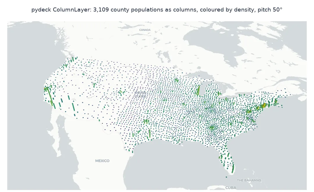
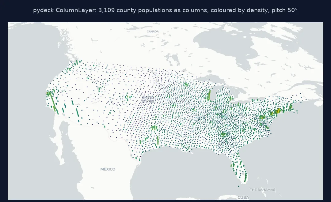
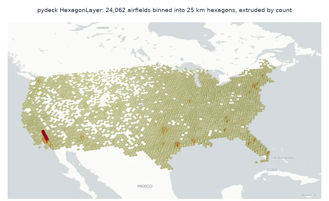
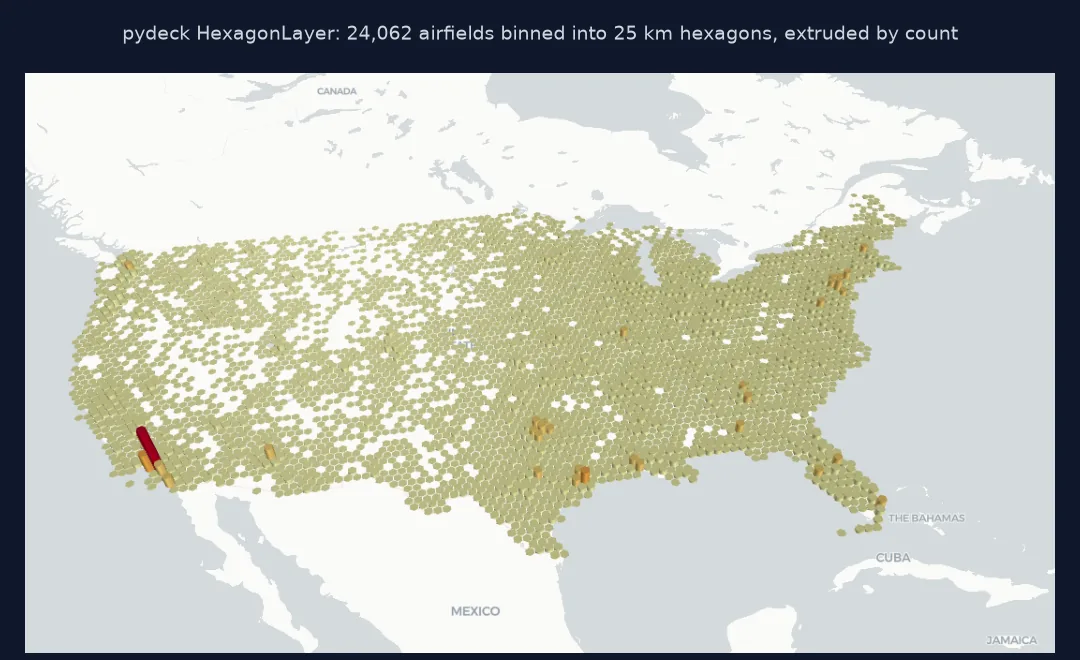
This page draws the 2023 population of every county in the conterminous US as 3D columns, aggregates 24,000 airfields in the conterminous US into extruded hexagons, colours the columns by density, fits the camera to the data, and saves each map as a standalone HTML file.

Quick answer

Build a layer from a DataFrame, set a tilted view, and save the deck:

import pydeck as pdk
layer = pdk.Layer("ColumnLayer", D, get_position=["lon", "lat"], get_elevation="POPESTIMATE2023", elevation_scale=0.04,
                  radius=9000, get_fill_color="rgb", pickable=True, auto_highlight=True)
view = pdk.ViewState(latitude=37.5, longitude=-96, zoom=3.6, pitch=50, bearing=-12)
deck = pdk.Deck(layers=[layer], initial_view_state=view, map_style="light", tooltip={"text": "{NAME}\n{pop_txt} people"})
deck.to_html("data/county_columns.html", open_browser=False, notebook_display=False)
print(f"columns: {len(D):,}; tallest {D.POPESTIMATE2023.max() * 0.04 / 1000:,.0f} km ({D.loc[D.POPESTIMATE2023.idxmax(), 'NAME']}); HTML {Path('data/county_columns.html').stat().st_size / 1e6:.2f} MB")

columns: 3,109; tallest 387 km (Los Angeles County, California); HTML 1.03 MB

The tallest of the 3,109 columns is Los Angeles County, at 387 km. The page is 1.03 MB.

Elevation scale, RGB colours, hexagons from points

1. Elevation scale

Heights are in metres: get_elevation times elevation_scale. With a scale of 1, Los Angeles County would be a column almost 10,000 km tall. Pick the scale from the largest value and the height you want it to have:

target_km = 400
scale = target_km * 1000 / D.POPESTIMATE2023.max()
print(f"largest value {D.POPESTIMATE2023.max():,}; scale for a {target_km} km column: {scale:.3f}")
print(f"median county at that scale: {D.POPESTIMATE2023.median() * scale / 1000:.1f} km tall")

largest value 9,663,345; scale for a 400 km column: 0.041
median county at that scale: 1.1 km tall

Los Angeles County's 9,663,345 people need a scale of 0.041 for a 400 km column, and at that scale the median county is just 1.1 km tall. That is the nature of a 3D column map: a few very large values dominate it.

2. Colours as RGB lists

deck.gl takes colours as [r, g, b] or [r, g, b, a] lists, not names or hex strings. Build them from a matplotlib colormap on log density:

print(f"first rows of the rgb column: {D.rgb.head(3).tolist()}")
print(f"density range coloured: {D.density_km2.min():.2f} to {D.density_km2.max():,.0f} people per km² on a log scale")

first rows of the rgb column: [[41, 121, 142], [50, 99, 141], [129, 211, 76]]
density range coloured: 0.02 to 17,227 people per km² on a log scale

Each row carries its own [r, g, b] list from the viridis colormap, across densities from 0.02 to 17,227 people per km² on a log scale.

3. Hexagons from points

HexagonLayer bins points into hexagons in the browser and extrudes each by its count. Aggregate all US airfields at a 25 km radius:

hexes = pdk.Layer("HexagonLayer", US, get_position=["longitude_deg", "latitude_deg"], radius=25000, elevation_scale=300,
                  elevation_range=[0, 1000], extruded=True, coverage=0.9, pickable=True)
deck2 = pdk.Deck(layers=[hexes], initial_view_state=pdk.ViewState(latitude=37.5, longitude=-96, zoom=3.6, pitch=45, bearing=10), map_style="light",
                 tooltip={"text": "{elevationValue} airfields"})
deck2.to_html("data/airfield_hexagons.html", open_browser=False, notebook_display=False)
print(f"points: {len(US):,}; HTML {Path('data/airfield_hexagons.html').stat().st_size / 1e6:.2f} MB")

points: 24,062; HTML 3.10 MB

All 24,062 points go into the page as JSON, 3.10 MB, three times the county page; the hexagon counts are computed in the browser.

Fitting the camera to the data

The data used on this page

The US Census Bureau's 2023 county cartographic boundaries and Vintage 2023 population estimates, reduced to one point per county inside its boundary, and every open place in the conterminous US from OurAirports. The light map style is CARTO's Positron vector basemap, which pydeck loads without a key.

from pathlib import Path

import geopandas as gpd
import matplotlib
import numpy as np
import pandas as pd
import requests

Path("data").mkdir(exist_ok=True)
def cached(path, url):
    p = Path(path)
    if not p.exists():
        r = requests.get(url, timeout=600)
        r.raise_for_status()
        p.write_bytes(r.content)
    return p
C = gpd.read_file(cached("data/cb_2023_us_county_20m.zip", "https://www2.census.gov/geo/tiger/GENZ2023/shp/cb_2023_us_county_20m.zip"))
est = pd.read_csv(cached("data/co-est2023-alldata.csv", "https://www2.census.gov/programs-surveys/popest/datasets/2020-2023/counties/totals/co-est2023-alldata.csv"),
                  encoding="latin-1", dtype={"STATE": str, "COUNTY": str})
est = est[est.SUMLEV == 50].assign(GEOID=lambda d: d.STATE + d.COUNTY)[["GEOID", "STNAME", "CTYNAME", "POPESTIMATE2023"]]
G = C[~C.STATEFP.isin(["02", "15", "72"])].merge(est, on="GEOID")
G["density_km2"] = G.POPESTIMATE2023 / (G.to_crs(5070).area / 1e6)
pt = G.to_crs(5070).representative_point().to_crs(4326)
D = pd.DataFrame({"NAME": G.CTYNAME + ", " + G.STNAME, "lon": pt.x, "lat": pt.y, "POPESTIMATE2023": G.POPESTIMATE2023, "density_km2": G.density_km2})
D["pop_txt"] = D.POPESTIMATE2023.map("{:,}".format)
norm = matplotlib.colors.LogNorm(vmin=max(D.density_km2.min(), 0.1), vmax=D.density_km2.max())
D["rgb"] = [[int(v * 255) for v in matplotlib.colormaps["viridis"](norm(d))[:3]] for d in D.density_km2]
A = pd.read_csv(cached("data/airports.csv", "https://davidmegginson.github.io/ourairports-data/airports.csv"), keep_default_na=False, na_values=[""])
US = A[(A.iso_country == "US") & (A.type != "closed") & A.longitude_deg.between(-130, -60) & A.latitude_deg.between(24, 50)][["ident", "longitude_deg", "latitude_deg"]]
print(f"{len(D):,} counties; {len(US):,} airfields in the conterminous US")

3,109 counties; 24,062 airfields in the conterminous US

The data is one point for each of the 3,109 counties, and 24,062 open airfields in the conterminous US.

Example 1: fit the camera to the data

pdk.data_utils.compute_view picks a centre and zoom that contain most of the points:

v = pdk.data_utils.compute_view(D[["lon", "lat"]], view_proportion=0.95)
print(f"computed view: latitude {v.latitude:.2f}, longitude {v.longitude:.2f}, zoom {v.zoom:.2f}")
v.pitch, v.bearing = 50, -12
deck.initial_view_state = v
deck.to_html("data/county_columns_fitted.html", open_browser=False, notebook_display=False)

computed view: latitude 38.28, longitude -91.66, zoom 2.00

compute_view centres the view at 38.28° N, 91.66° W with zoom 2.00. That is wider than the zoom of 3.6 chosen by hand, so check a computed view before using it.

pydeck writes a deck.gl description into a page

pydeck builds a JSON description of a deck.gl visualisation (layers, data, view state, basemap) and writes it into an HTML page that loads deck.gl from a CDN. The data travels inside the page as JSON, so the file grows with the number of rows and columns passed to each layer. deck.gl draws on the GPU with WebGL, which is why it can extrude thousands of columns and still rotate smoothly. Layer properties starting with get_ are accessors, read per row from a column name or an expression, while others such as radius and elevation_scale apply to the whole layer.

3D adds a dimension but also hides things. Tall columns block the ones behind them, the tilt makes distant columns smaller, and heights are hard to compare across the screen. A 3D map works best for a single striking quantity, such as where the people are, and should be checked against a flat map or a table. Aggregating layers like HexagonLayer compute in the browser, so their counts are not available in Python. To report the numbers, compute the same bins with H3 or a grid.

Mapbox styles, tilting and large data

• Mapbox styles: Mapbox map styles need an API key passed as api_keys={"mapbox": ...}; the CARTO styles light, dark and road do not.
• Hold Ctrl and drag (or right-drag) to rotate and tilt in the browser.
• Large data: for hundreds of thousands of points, pass only the columns needed, or use lonboard, which sends binary data instead of JSON.
• Jupyter: deck.show() displays inline; to_html(notebook_display=False) writes a file without displaying.

Internal links

• How to make an interactive arc map of flows with pydeck — another deck.gl layer
• How to map a million points with lonboard in Python — deck.gl with binary data
• How to render a million points in a map app with pydeck — performance in apps

FAQ

How do I make a 3D map in Python?

Use pydeck with a ColumnLayer or HexagonLayer, set pitch in the ViewState to tilt the view, and save with deck.to_html().

How do I set colours in pydeck?

Give colours as lists of [r, g, b] or [r, g, b, a] integers from 0 to 255, either fixed or from a DataFrame column.

Why are my pydeck columns too tall or invisible?

Heights are in metres; set elevation_scale so the largest value gives a height of a few hundred kilometres at a national scale.

Does pydeck need a Mapbox token?

Only for Mapbox styles; the built-in CARTO styles work without one.