
Yield monitor data explained: what the numbers really are
Problem statement
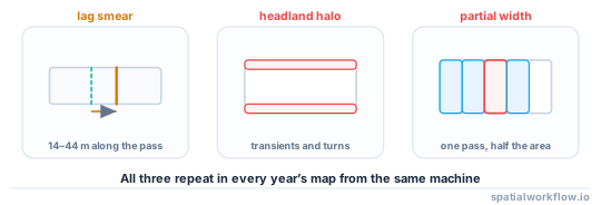
A yield map looks like a measurement of the field. It is a measurement of a machine moving through the field, and the difference produces artefacts that dominate the map if they are not removed: a stripe along every start and stop, a halo at every headland turn, a band down every pass where the header was not full, and a smear of about twenty metres wherever the crop changed.
None of these is noise in the statistical sense. They are systematic, they repeat in every year's map from the same machine, and a clustering algorithm will happily build management zones out of them.
This guide explains where each artefact comes from, which of them can be corrected and which can only be removed.
Quick answer
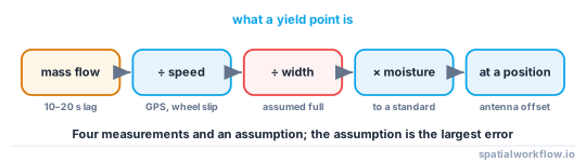
A yield point is a mass flow measured at the top of the elevator, divided by an area inferred from speed and an assumed header width:
yield = mass_flow / (speed × effective_width × moisture_correction)
Every term contributes an error:
| term | error | effect on the map |
|---|---|---|
| mass flow | sensor lag of 10–20 s | yield attributed 20–60 m behind where it grew |
| speed | GPS noise, wheel slip | spikes at low speed, stripes at changes |
| effective width | assumed full, often is not | a band of inflated yield down every partial pass |
| moisture | measured or assumed | a systematic offset between passes |
| position | receiver offset from the header | the whole map shifted by metres |
Step-by-step solution
1. Understand the lag
Grain takes ten to twenty seconds to travel from the header to the mass-flow sensor. At a typical 5 km/h that is 14–28 m, and at 8 km/h it is 22–44 m. Unless the data has been lag-corrected, every value is attributed to ground the machine had already left — which smears every real boundary in the direction of travel.
2. Understand the partial-width problem
The monitor assumes the full header width unless the operator tells it otherwise. On the last pass of a land, around obstacles and on tapered headlands, the header is part full, so the same grain flow is divided by too large an area and the recorded yield is too low — or, where the machine overlaps a previous pass, grain is counted twice over ground already cut.
3. Understand the start and stop transients
Flow builds up over several seconds after the machine starts moving and decays after it stops. Points recorded during either are meaningless, and they cluster at the ends of every pass, which is exactly where headland zones get drawn.
4. Understand the moisture correction
Yield is reported at a standard moisture. If the moisture sensor is out or the correction is applied inconsistently between passes, whole passes shift relative to each other by several percent, producing stripes that follow the machine rather than the field.
5. Understand the position offset
The GNSS antenna is on the cab roof, the crop entered the header several metres ahead. A constant offset moves the entire map, which matters when comparing with a prescription or a soil sample.
6. Know which artefacts can be corrected
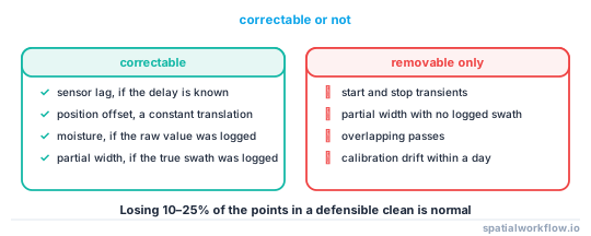
- Lag — correctable if the delay is known, by shifting values back along the track.
- Position offset — correctable with a constant translation.
- Moisture — correctable if the raw moisture is recorded.
- Partial width — correctable only if the true swath width was logged; otherwise the affected points have to go.
- Start/stop transients — not correctable; remove them.
7. Expect to remove a substantial fraction of the points
A defensible cleaning pass removes start and stop transients, overlapping passes, extreme speeds, extreme flows and impossible yields. Losing 10–25% of the points is normal, and the number should be reported.
Code examples
Example 1 — what a raw yield file contains
import pandas as pd, numpy as np, geopandas as gpd

y = pd.read_csv("harvest_2025.csv")
print(y.columns.tolist())
print(y[["yield_t_ha", "speed_kmh", "swath_m", "moisture_pct", "flow_kg_s"]]
      .describe(percentiles=[.01, .5, .99]).round(2))

print(f"\npoints {len(y):,}")
print(f"zero or negative yield: {(y.yield_t_ha <= 0).sum():,}")
print(f"speed under 1 km/h: {(y.speed_kmh < 1).sum():,}")
print(f"swath less than full: {(y.swath_m < y.swath_m.max()).mean():.1%}")
The last line is the one that surprises people. A quarter to a third of points recorded at less than full header width is normal, and every one of them has an area error.
Example 2 — reconstruct the geometry of each pass
import numpy as np, pandas as pd, geopandas as gpd

def add_pass_geometry(y, heading_col="heading_deg", gap_s=10):
    y = y.sort_values("timestamp").copy()
    dt = y["timestamp"].diff().dt.total_seconds()
    turn = y[heading_col].diff().abs().mod(360)
    turn = np.minimum(turn, 360 - turn)
    y["pass_id"] = ((dt > gap_s) | (turn > 60)).cumsum()

    sizes = y.groupby("pass_id").size()
    print(f"{len(sizes):,} passes, median {sizes.median():.0f} points, "
          f"{int((sizes < 10).sum()):,} passes with fewer than 10 points")

    y["point_in_pass"] = y.groupby("pass_id").cumcount()
    y["from_end"] = y.groupby("pass_id")["point_in_pass"].transform("max") - y["point_in_pass"]
    return y
Once the passes are reconstructed, the start and stop transients are the first and last few points of each one, and the headland is where the passes turn.
Example 3 — correct the lag
import numpy as np, pandas as pd

def correct_lag(y, lag_s=12.0):
    """Shift each yield value back along its own pass by the sensor delay."""
    out = []
    for pid, g in y.groupby("pass_id", sort=False):
        g = g.sort_values("timestamp").copy()
        t = (g["timestamp"] - g["timestamp"].iloc[0]).dt.total_seconds().values
        shifted = np.interp(t, t - lag_s, g["yield_t_ha"].values,
                            left=np.nan, right=np.nan)
        g["yield_lag_corrected"] = shifted
        out.append(g)
    return pd.concat(out)

y = correct_lag(y, lag_s=12.0)
moved = (y["yield_t_ha"] - y["yield_lag_corrected"]).abs()
print(f"median change from lag correction: {moved.median():.2f} t/ha")
The lag is a machine constant that can be estimated by cross-correlating the yield signal against a known boundary — the edge of a trial strip, or a change of variety — and the estimate is worth making once per combine rather than taking a default.
Explanation
Why the lag smears boundaries rather than shifting them
If the delay were constant in distance, the map would simply be translated. It is constant in time, so the distance depends on the speed, which varies within and between passes. A boundary is therefore displaced by different amounts in different places, which blurs it rather than moving it — and it is why a lag-uncorrected map cannot resolve a trial strip narrower than about forty metres.
Why partial width is the largest single error
The monitor divides a measured mass by an assumed area. If the header is half full and the monitor assumes it is full, the recorded yield is half the true value — a 50% error, far larger than anything the sensors contribute. It happens on every last pass, around every obstacle and on every tapered headland, which in an irregular field can be a quarter of the points.
Why moisture produces stripes
The reported yield is corrected to a standard moisture, typically 15% for cereals. If the moisture reading drifts or the correction is applied from a manual entry that was changed part way through the day, the correction differs between passes cut at different times. The result is a stripe pattern aligned with the machine's direction rather than with anything in the field.
Why these artefacts survive into management zones
They are spatially structured: headlands are at the edges, partial passes are along one side, start-stop transients are in rows. Clustering finds spatial structure, so a zoning built on uncleaned yield data reproduces the harvest pattern. The give-away is a zone boundary that runs parallel to the direction of travel.
Edge cases or notes
- Formats vary by manufacturer. A yield file is a vendor format with a common shape.
- Multiple harvests in one file. Split by date before anything else.
- Two combines in one field have two lags and two calibrations.
- Calibration drift within a day is common.
- Grain cart weights are the reference. Scale the map to the weighbridge total.
- Dry and wet grain are different products. Record the moisture basis.
- The first year of a new monitor is the worst. Calibration improves.
- Report the cleaning statistics. Removing 20% of points is a result.
Internal links
- How to clean yield monitor data in Python — the cleaning pipeline
- A yield map has impossible values and stripes — the symptoms in detail
- Management zones explained — why uncleaned yield makes bad zones
- How to analyse an on-farm strip trial in Python — where the lag limits resolution
- How to remove spatial outliers in Python — the statistical half of cleaning
- How to clean a GPS track in Python — reconstructing the passes
- GPS error explained — the position component
- How to write a variable-rate prescription map — what the cleaned map feeds
FAQ
What does a yield monitor actually measure?
Mass flow at the top of the clean grain elevator, divided by an area inferred from ground speed and an assumed header width, corrected to a standard moisture.
Why is my yield map smeared along the direction of travel?
Sensor lag. Grain takes ten to twenty seconds to reach the sensor, which at 5–8 km/h is 14–44 m of travel.
Why are there stripes down my field?
Usually partial header width being recorded as full width, or an inconsistent moisture correction between passes cut at different times.
Why is the headland always different?
Start and stop transients, turning, and partial width all concentrate there. Headland points are the least reliable in the file.
How many points should I expect to remove?
Ten to twenty-five per cent is normal for a defensible cleaning pass. Report the number.
Can I fix all of this?
Lag, position offset and moisture are correctable if the raw values were logged. Partial width is correctable only if the true swath was recorded; start and stop transients can only be removed.