How to Measure the Effect of the Clock Change on Road Crashes in Python

On this page

Problem statement

Twice a year the clocks move an hour and an hour of daylight moves with them. In November, when US clocks go back, the evening rush hour falls into darkness overnight; in March it moves back into daylight. If darkness matters to crash risk, the effect should show as a step in evening crashes in the week of the change, much larger than any week-to-week drift. This is a natural experiment in the data: the date, not the weather or the season, decides when the light changes.

This page assembles seven years of FARS crash files, 2017–2023, finds the daylight saving time transitions, compares fatal crashes in the evening rush hour, 17:00–19:59, in the weeks before and after each change, and separates crashes involving pedestrians.

Quick answer

Stack the crash files, locate each transition date, and count crashes by week relative to it:

rows = []
for year in YEARS:
    for season, change in (("March", nth_sunday(year, 3, 2)), ("November", nth_sunday(year, 11, 1))):
        for week in range(-3, 4):
            w = A[(A.date >= change + pd.Timedelta(weeks=week)) & (A.date < change + pd.Timedelta(weeks=week + 1))]
            ev = w[w.HOUR.between(17, 19)]
            rows.append({"season": season, "week": week, "evening": len(ev), "evening_ped": int((ev.PEDS > 0).sum())})
W = pd.DataFrame(rows).groupby(["season", "week"]).sum()
print(W.unstack("season").to_string())

       evening          evening_ped         
season   March November       March November
week                                        
-3         829      937         294      251
-2         830      970         274      332
-1         816      967         262      337
 0         687     1147         113      477
 1         636     1095         100      456
 2         647     1100          93      475
 3         644     1097          97      483

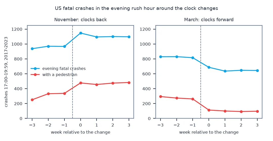
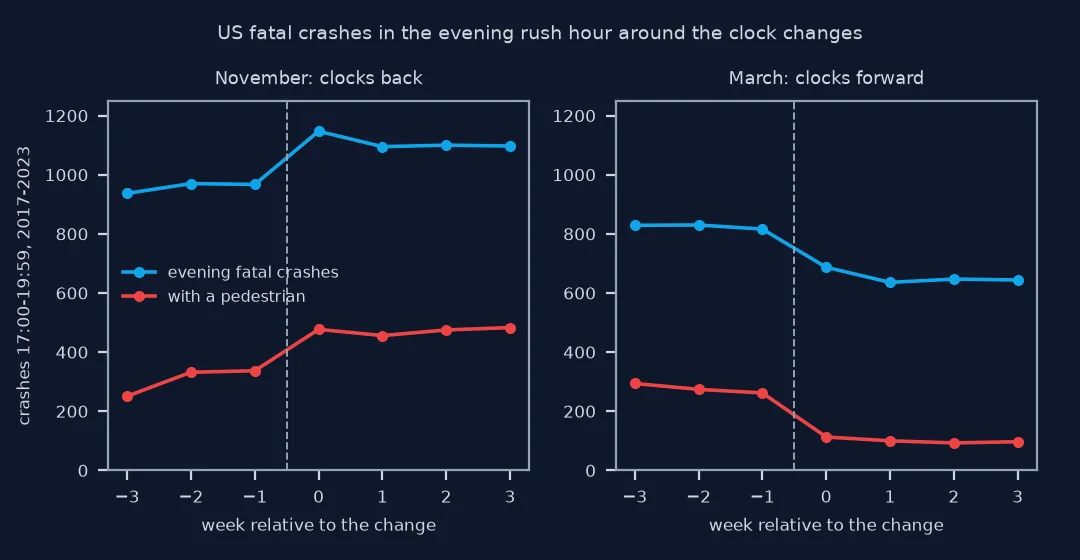
Summed over seven years, the evening rush hour had about 950 fatal crashes in each of the three weeks before the November change and 1,147 in the week of it, staying near 1,100 afterwards. In March the step goes the other way, from about 825 to 687.

Two line charts of US fatal crashes between 17:00 and 19:59, summed over 2017 to 2023, for the three weeks before and after each clock change: in November evening crashes step up from about 950 a week to 1,147 in the week of the change and stay near 1,100, and those with a pedestrian from about 300 to 477; in March they step down from about 825 to 687 and stay near 640, and those with a pedestrian from about 275 to 113. — Evening crashes around the clock changes.

Stack years, measure each seasonal step, check it is light

1. Stack several years of FARS

The zip layout and the capitalisation of file and column names changed over the years, and the 2021 and 2022 files begin with a byte-order mark that turns the first column name into ï»¿STATE when read as Latin-1; find the crash file by name and clean the column names:

print(A.groupby("YEAR").size().to_string())
print(f"crashes with an unusable date: {N_BAD}; with unknown hour: {(A.HOUR > 23).sum()}")

YEAR
2017    34560
2018    33919
2019    33487
2020    35935
2021    39785
2022    39422
2023    37769
crashes with an unusable date: 0; with unknown hour: 1902

254,877 fatal crashes from seven files; every record has a valid date, and 1,902 have an unknown hour, which the hourly windows leave out.

2. Measure the step in each season

Compare the transition week with the average of the three weeks before it:

for season in ("November", "March"):
    s = W.loc[season]
    before = s.loc[-3:-1].mean()
    print(f"{season}: evening crashes {s.loc[0, 'evening'] / before['evening'] - 1:+.0%} in the week of the change; "
          f"with a pedestrian {s.loc[0, 'evening_ped'] / before['evening_ped'] - 1:+.0%}; "
          f"weeks +1 to +3 {s.loc[1:3, 'evening'].mean() / before['evening'] - 1:+.0%}")

November: evening crashes +20% in the week of the change; with a pedestrian +56%; weeks +1 to +3 +15%
March: evening crashes -17% in the week of the change; with a pedestrian -59%; weeks +1 to +3 -22%

Against the three weeks before, the November change brings 20% more evening crashes and 56% more evening crashes with a pedestrian; the level stays 15% higher for the following three weeks. The March change brings 17% fewer, and 59% fewer with a pedestrian.

The size of the step.

3. Check it is the light, not the week

If the step came from darkness, the crashes that move should be crashes in the dark. Count evening crashes by light condition:

dark_codes = [2, 3, 6]                                                  # dark: not lighted, lighted, unknown lighting
for season in ("November", "March"):
    sel = []
    for year in YEARS:
        d = nth_sunday(year, 11, 1) if season == "November" else nth_sunday(year, 3, 2)
        for week, label in ((-1, "week before"), (0, "week of change")):
            w = A[(A.date >= d + pd.Timedelta(weeks=week)) & (A.date < d + pd.Timedelta(weeks=week + 1)) & A.HOUR.between(17, 19)]
            sel.append({"when": label, "dark": int(w.LGT_COND.isin(dark_codes).sum()), "all": len(w)})
    t = pd.DataFrame(sel).groupby("when").sum()
    print(f"{season}: dark share of evening crashes {t.loc['week before', 'dark'] / t.loc['week before', 'all']:.0%} -> "
          f"{t.loc['week of change', 'dark'] / t.loc['week of change', 'all']:.0%}")

November: dark share of evening crashes 63% -> 82%
March: dark share of evening crashes 64% -> 21%

The share of evening crashes in the dark jumps from 63% to 82% in November and falls from 64% to 21% in March: the crashes that move are the ones that change light.

The morning side of the trade

The data used on this page

NHTSA's FARS national CSV files for 2017 to 2023, crash level. US daylight saving time starts on the second Sunday of March and ends on the first Sunday of November; Arizona and Hawaii do not observe it, and their crashes are left in, which dilutes the effect slightly.

import zipfile
from pathlib import Path

import pandas as pd
import requests

Path("data").mkdir(exist_ok=True)
YEARS = range(2017, 2024)
frames = []
for year in YEARS:
    f = Path(f"data/FARS{year}NationalCSV.zip")
    if not f.exists():
        f.write_bytes(requests.get(f"https://static.nhtsa.gov/nhtsa/downloads/FARS/{year}/National/FARS{year}NationalCSV.zip", timeout=600).content)
    z = zipfile.ZipFile(f)
    name = next(n for n in z.namelist() if n.lower().endswith("accident.csv"))
    clean = lambda c: c.replace("ï»¿", "").upper()                     # 2021 and 2022 start with a byte-order mark
    a = pd.read_csv(z.open(name), encoding="latin1", low_memory=False,
                    usecols=lambda c: clean(c) in {"STATE", "ST_CASE", "YEAR", "MONTH", "DAY", "HOUR", "FATALS", "LGT_COND", "PEDS"})
    frames.append(a.rename(columns=clean))
A = pd.concat(frames, ignore_index=True)
A["date"] = pd.to_datetime(dict(year=A.YEAR, month=A.MONTH, day=A.DAY), errors="coerce")
N_BAD = int(A.date.isna().sum())
A = A.dropna(subset=["date"])


def nth_sunday(year, month, n):
    first = pd.Timestamp(year, month, 1)
    return first + pd.Timedelta(days=(6 - first.weekday()) % 7) + pd.Timedelta(weeks=n - 1)


print(f"{len(A):,} fatal crashes, {A.YEAR.min()}-{A.YEAR.max()}; November 2023 change: {nth_sunday(2023, 11, 1):%d %b}, March 2023: {nth_sunday(2023, 3, 2):%d %b}")

254,877 fatal crashes, 2017-2023; November 2023 change: 05 Nov, March 2023: 12 Mar

Example 1: the morning, the other side of the trade

The clock change moves light from the evening to the morning in November and back in March. Count the morning rush hour, 06:00–08:59, the same way:

for season, (m, n) in (("November", (11, 1)), ("March", (3, 2))):
    before, after = [], []
    for year in YEARS:
        d = nth_sunday(year, m, n)
        morning = A[A.HOUR.between(6, 8)]
        before.append(((morning.date >= d - pd.Timedelta(weeks=3)) & (morning.date < d)).sum() / 3)
        after.append(((morning.date >= d) & (morning.date < d + pd.Timedelta(weeks=1))).sum())
    print(f"{season}: morning crashes in the week of the change {sum(after) / sum(before) - 1:+.0%} against the three weeks before")

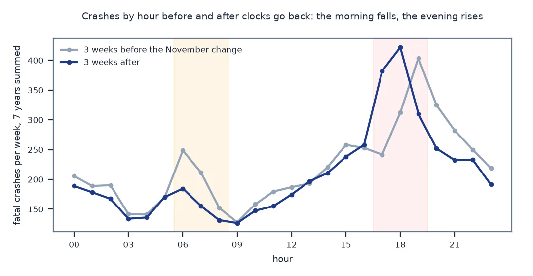
November: morning crashes in the week of the change -24% against the three weeks before
March: morning crashes in the week of the change +26% against the three weeks before

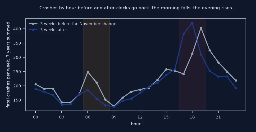
The morning mirrors the evening: 24% fewer crashes in the November week, as mornings become lighter, and 26% more in March, as they become dark again.

Line chart of fatal crashes by hour per week for the three weeks before and after the November change, summed over 2017 to 2023: after the change the morning peak around 06:00 to 08:00 falls, and the evening peak moves an hour earlier, from 19:00 to 18:00, and rises. — The daily profile shifts with the light.

A shift in light and little else

One hour of light, moved twice a year.

The clock change is useful because it shifts light without shifting anything else much: the weather, traffic volumes and the time of year change gradually, but at 18:00 on the Monday after the November change it is dark where the Friday before it was dusk. A step that appears exactly at the change and stays is evidence about light; slow drift across the weeks is the season.

In FARS the evening step is large and clear in both directions. After the November change evening fatal crashes rise sharply and stay higher, while the share in the dark jumps; crashes involving pedestrians rise most, consistent with drivers failing to see people on foot. In March the reverse happens. The morning moves the other way by a similar proportion, a quarter down in November and a quarter up in March, on smaller numbers of crashes.

Two cautions. Counting crashes in a fixed clock window across the change compares different solar times, which is the point here but matters when comparing with other studies. And this design shows the effect of light on the timing of crashes; whether permanent daylight saving time would reduce deaths overall depends on the balance between mornings and evenings over the whole year, which needs a different analysis.

Arizona and Hawaii, 2020 and week alignment

Clock change traps.

Arizona and Hawaii: no clock change; dropping them sharpens the estimate slightly.
2020: the pandemic changed traffic in spring 2020; the March 2020 change fell days before lockdowns, and a sensitivity check without 2020 is worth running.
Week alignment: weeks here run Sunday to Saturday from the change, so the transition week starts with the shortened or lengthened Sunday.
Time zones: FARS hours are local time, which is what matters for light.
Other years: before 2007 the US changed clocks on different dates; adjust nth_sunday for older data.

Internal links

How to map fatal road crashes in the US with FARS in Python — the FARS files and light conditions
How to analyse pedestrian deaths with FARS in Python — pedestrians and darkness

FAQ

Do road deaths increase after the clocks go back?

In FARS 2017–2023, fatal crashes in the evening rush hour rose by 20% in the week after the November change, and those involving a pedestrian by 56%.

How do I find daylight saving time dates in Python?

In the US since 2007, the change is on the second Sunday of March and the first Sunday of November; compute them from the first day of the month and the weekday.

Why do pedestrian crashes rise in November?

Because the evening commute moves into darkness overnight; the share of evening fatal crashes in the dark rises from 63% to 82% in the week of the change.

Does the spring clock change cause crashes?

In FARS 2017–2023, evening crashes fell by 17% in the week after the March change, as the evening rush hour returned to daylight, while morning crashes rose by 26%.