How to Find Clusters of Fatal Crashes with DBSCAN in Python

On this page

Problem statement

Road safety engineers look for crash clusters: short stretches of road or single junctions where several serious crashes happened within a few years. Unlike a high-injury network, which ranks every street, cluster detection asks which points sit unusually close together. DBSCAN does exactly that, grouping points with enough neighbours within a distance and leaving the rest as noise, and it works directly on latitude and longitude with a haversine distance. Its two parameters decide what counts as a cluster, and the clusters are only worth acting on if crashes keep happening there.

This page runs DBSCAN on five years of fatal crashes in Harris County, Texas, from FARS, compares parameter settings, names the clusters by the road the crashes were on, and tests whether clusters found in 2019–2021 caught more of the 2022–2023 crashes than their area would suggest.

Quick answer

Convert coordinates to radians, set eps to a distance divided by the Earth's radius, and fit with the haversine metric:

X = np.radians(H[["LATITUDE", "LONGITUD"]].to_numpy())
labels = DBSCAN(eps=300 / 6_371_000, min_samples=5, metric="haversine").fit_predict(X)
H["cluster"] = labels
print(f"{len(H):,} fatal crashes in Harris County, 2019-2023; {labels.max() + 1} clusters; {(labels >= 0).mean():.1%} of crashes in one")
C = H[H.cluster >= 0].groupby("cluster").agg(crashes=("ST_CASE", "size"), deaths=("FATALS", "sum"), road=("TWAY_ID", lambda r: r.mode()[0]))
print(C.sort_values("crashes", ascending=False).head(6).to_string())

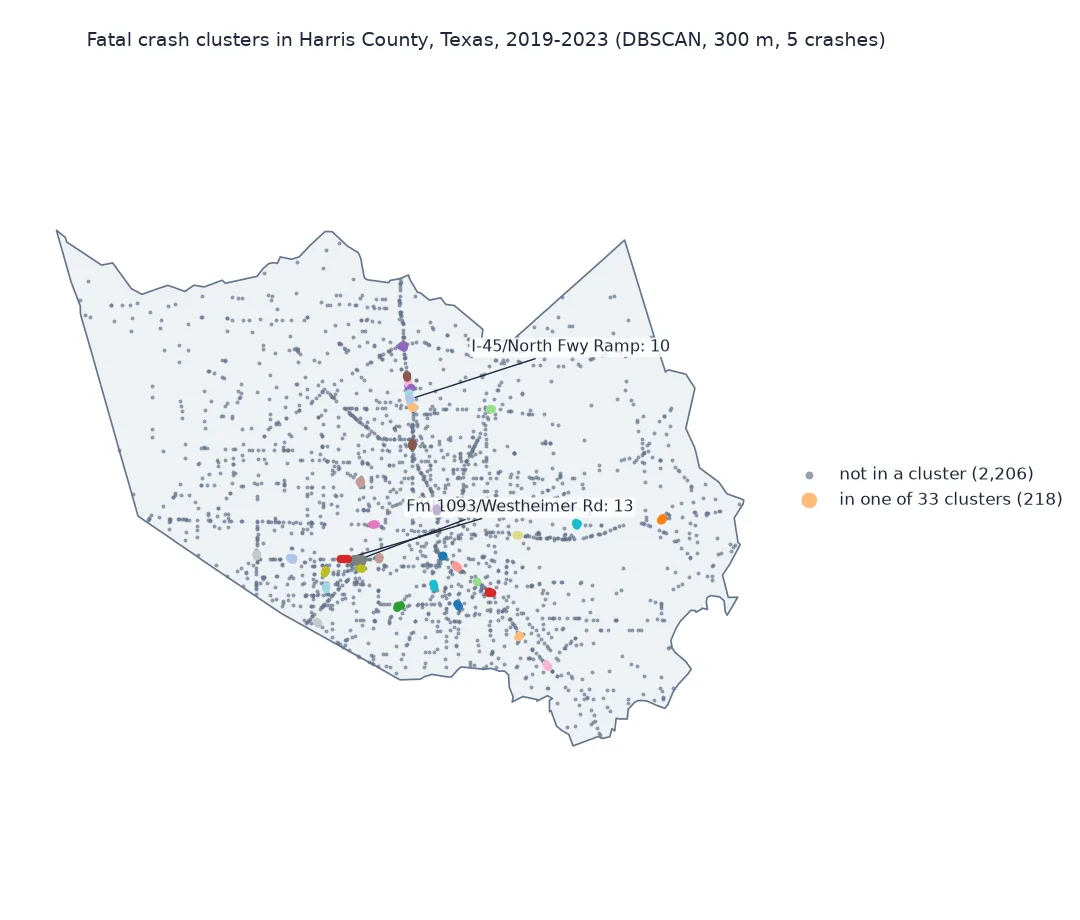
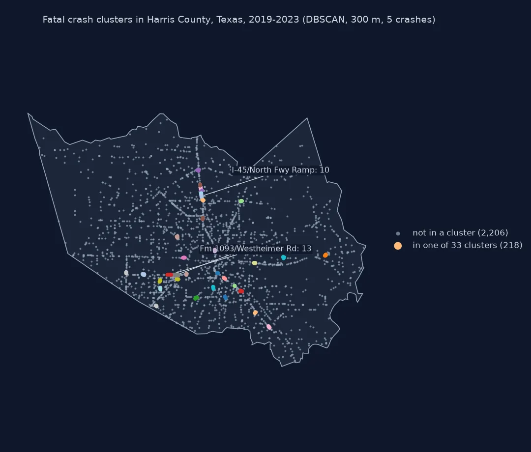
2,424 fatal crashes in Harris County, 2019-2023; 33 clusters; 9.0% of crashes in one
         crashes  deaths                    road
cluster                                         
23            16      19           WESTHEIMER RD
11            13      13   FM 1093/WESTHEIMER RD
3             10      10     I-45/NORTH FWY RAMP
24             9       9                    SR-6
7              8       9  I-610/INDEPENDENCE PKY
4              8       8                    I-10

Five fatal crashes within 300 metres of each other, over five years, define 33 clusters holding 9.0% of Harris County's 2,424 fatal crashes. The largest, 16 crashes and 19 deaths, and two more of the top seven are on Westheimer Road, a long commercial arterial; most of the others are on interstates, their ramps and state highways.

Map of Harris County, Texas, with 2,424 fatal crashes from 2019 to 2023: 2,206 not in any cluster as small grey dots tracing the freeways and arterials, and 218 in 33 DBSCAN clusters as coloured groups, several on Westheimer Road in the south-west, with 13 crashes in one, and along I-45 north of downtown, with 10 at a ramp. — Fatal crash clusters in Harris County.

Area and clean coordinates, parameter settings, later years

1. Select the area and clean the coordinates

FARS coordinates carry codes for missing values; keep valid ones only:

print(f"Harris County crashes 2019-2023: {len(HC):,}; with valid coordinates: {len(H):,}")
print(H.groupby("YEAR").size().to_string())

Harris County crashes 2019-2023: 2,428; with valid coordinates: 2,424
YEAR
2019    397
2020    456
2021    540
2022    527
2023    504

Four crashes have coded coordinates and are left out. Fatal crashes in the county rose from 397 in 2019 to 540 in 2021 before easing.

2. Compare parameter settings

eps is the neighbourhood radius and min_samples the number of crashes, including the point itself, needed to start a cluster:

for eps_m, k in ((200, 4), (300, 5), (500, 8), (1000, 10)):
    lab = DBSCAN(eps=eps_m / 6_371_000, min_samples=k, metric="haversine").fit_predict(X)
    print(f"eps {eps_m:>4} m, min_samples {k:>2}: {lab.max() + 1:>3} clusters, {(lab >= 0).mean():5.1%} of crashes in clusters")

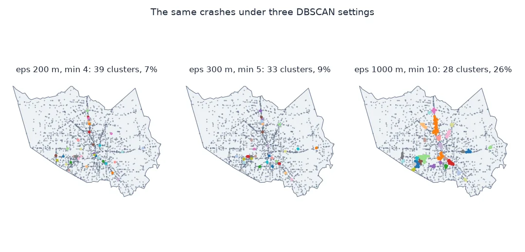
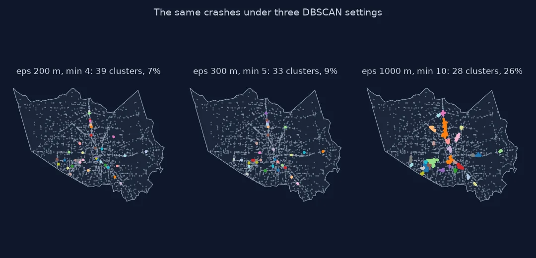
eps  200 m, min_samples  4:  39 clusters,  7.5% of crashes in clusters
eps  300 m, min_samples  5:  33 clusters,  9.0% of crashes in clusters
eps  500 m, min_samples  8:  16 clusters,  7.5% of crashes in clusters
eps 1000 m, min_samples 10:  28 clusters, 26.4% of crashes in clusters

The setting matters less than expected between 200 and 500 metres, 7.5% to 9.0% of crashes in 16 to 39 clusters, and a lot beyond: at a kilometre, clusters start to swallow whole corridors and a quarter of all crashes.

Three maps of the same Harris County fatal crashes clustered with different DBSCAN settings: eps 200 metres and minimum 4 gives 39 small clusters with 7 percent of crashes; eps 300 metres and minimum 5 gives 33 clusters with 9 percent; eps 1,000 metres and minimum 10 gives 28 large clusters along whole freeway stretches with 26 percent. — Three parameter settings.

3. Test the clusters on later years

Fit on 2019–2021, buffer each cluster's crashes by the same 300 metres, and count how many 2022–2023 crashes fall inside, against the share of the county's land the buffers cover:

early, late = H[H.YEAR <= 2021], H[H.YEAR >= 2022]
lab = DBSCAN(eps=300 / 6_371_000, min_samples=5, metric="haversine").fit_predict(np.radians(early[["LATITUDE", "LONGITUD"]].to_numpy()))
pts = gpd.GeoSeries(gpd.points_from_xy(early.LONGITUD, early.LATITUDE), crs=4326).to_crs(32615)
zones = pts[lab >= 0].buffer(300).union_all()
lp = gpd.GeoSeries(gpd.points_from_xy(late.LONGITUD, late.LATITUDE), crs=4326).to_crs(32615)
hit = lp.within(zones).mean(); area = zones.area / COUNTY.area
print(f"clusters from 2019-2021: {lab.max() + 1}, holding {(lab >= 0).sum()} of {len(early):,} crashes; they cover {area:.2%} of the county")
print(f"2022-2023 crashes inside them: {hit:.1%}; ratio to area share {hit / area:.0f}x")

clusters from 2019-2021: 5, holding 26 of 1,393 crashes; they cover 0.06% of the county
2022-2023 crashes inside them: 1.0%; ratio to area share 16x

Three years of fatal crashes give only five clusters, covering 0.06% of the county. They caught 1.0% of the next two years' crashes, sixteen times their area share: the places persist, but at this severity there are few of them, and injury crashes would give a far denser test.

What the crash clusters are made of

The data used on this page

NHTSA's FARS national files for 2019 to 2023, crashes in Harris County, Texas (state 48, county 201), and the Census Bureau's 2023 cartographic boundary file for counties. Distances are measured on UTM zone 15N (EPSG:32615) for the buffers.

import zipfile
from pathlib import Path

import geopandas as gpd
import numpy as np
import pandas as pd
import requests
from sklearn.cluster import DBSCAN

Path("data").mkdir(exist_ok=True)
frames = []
for year in range(2019, 2024):
    f = Path(f"data/FARS{year}NationalCSV.zip")
    if not f.exists():
        f.write_bytes(requests.get(f"https://static.nhtsa.gov/nhtsa/downloads/FARS/{year}/National/FARS{year}NationalCSV.zip", timeout=600).content)
    z = zipfile.ZipFile(f)
    a = pd.read_csv(z.open(next(n for n in z.namelist() if n.lower().endswith("accident.csv"))), encoding="latin1", low_memory=False)
    a.columns = [c.replace("ï»¿", "").upper() for c in a.columns]          # byte-order mark in some years
    frames.append(a[["STATE", "COUNTY", "ST_CASE", "YEAR", "FATALS", "LATITUDE", "LONGITUD", "TWAY_ID"]])
A = pd.concat(frames, ignore_index=True)
HC = A[(A.STATE == 48) & (A.COUNTY == 201)]
H = HC[~HC.LATITUDE.isin([77.7777, 88.8888, 99.9999]) & ~HC.LONGITUD.isin([777.7777, 888.8888, 999.9999])].copy()
G = Path("data/cb_2023_us_county_5m.zip")
if not G.exists():
    G.write_bytes(requests.get("https://www2.census.gov/geo/tiger/GENZ2023/shp/cb_2023_us_county_5m.zip", timeout=300).content)
COUNTY = gpd.read_file(G).query("GEOID == '48201'").to_crs(32615).geometry.iloc[0]
print(f"{len(A):,} US fatal crashes 2019-2023; Harris County {COUNTY.area / 1e6:,.0f} km²")

186,398 US fatal crashes 2019-2023; Harris County 4,593 km²

Example 1: what the clusters are made of

Clusters along one road and clusters around one junction look alike on a map. Count how many distinct roads each cluster's crashes were recorded on:

roads = H[H.cluster >= 0].groupby("cluster").TWAY_ID.agg(lambda r: r.str.replace(r"\s+", " ", regex=True).nunique())
print(f"clusters on a single named road: {(roads == 1).sum()} of {len(roads)}; median roads per cluster: {roads.median():.0f}")
interstate = H[H.cluster >= 0].TWAY_ID.str.contains(r"^I-|\bIH\b", regex=True).mean()
print(f"crashes in clusters recorded on an interstate: {interstate:.0%}; all Harris County crashes: {H.TWAY_ID.str.contains(r'^I-|IH', regex=True).mean():.0%}")

clusters on a single named road: 0 of 33; median roads per cluster: 4
crashes in clusters recorded on an interstate: 45%; all Harris County crashes: 21%

No cluster's crashes are all recorded on a single road name: the median cluster mixes four, from junctions with cross streets, ramps and spelling variants. 45% of clustered crashes are on interstates, against 21% of all crashes.

Clusters tested on later years.

How DBSCAN defines a cluster

Choosing parameters.

DBSCAN defines a cluster by density: a point with at least min_samples points within eps of it is a core point, points within eps of a core point join its cluster, and everything else is noise. It needs no number of clusters in advance and leaves isolated crashes alone, which suits crash data, where most crashes are scattered and only a few places stand out. The haversine metric measures great-circle distance on coordinates in radians, so eps is a distance divided by the Earth's radius.

The parameters encode a definition of a crash cluster: five fatal crashes within 300 metres over five years is a stricter test than four within 200 metres, and much stricter than ten within a kilometre, which starts merging whole corridors. There is no correct setting; there is a setting that matches the question and the scale of the interventions on offer, such as a junction redesign or a corridor programme. The temporal test makes the result defensible: zones drawn from three years that catch a disproportionate share of the next two years' crashes are places, not coincidences.

Sparse fatal crashes and divided highways

Crash cluster traps.

Fatal crashes are sparse: with injury crashes, clusters become denser and more stable; FARS is used here because it is national and open.
Projected alternative: DBSCAN with Euclidean distance on projected metres gives nearly the same result at a county scale.
Road names: TWAY_ID is free text, with variants such as "I-45" and "IH-45"; normalise before grouping.
Divided highways: crashes on opposite carriageways can join one cluster; split by direction of travel if that matters.
Exposure: a cluster on a road carrying 200,000 vehicles a day may be safer per vehicle than a quiet one; traffic counts give the rate.

Internal links

How to cluster points by location with DBSCAN in Python — DBSCAN in general
DBSCAN returns one giant cluster or labels everything noise — choosing parameters
How to build a high-injury network from crash data in Python — ranking every street instead

FAQ

How do I cluster crash locations with DBSCAN in Python?

Convert latitude and longitude to radians, use DBSCAN(eps=metres / 6371000, min_samples=k, metric="haversine"), and treat label -1 as noise.

What eps should I use for crash clusters?

It depends on the intervention: 100 to 300 metres for junctions and short stretches, longer for corridors; compare several and test the clusters on later years.

Are crash clusters real or random?

Test them on later years: the five clusters found in Harris County's 2019–2021 fatal crashes covered 0.06% of the county and caught 1.0% of the 2022–2023 crashes, sixteen times their area share, though few crashes in absolute terms.

Why are so many crashes labelled noise?

Because most fatal crashes are isolated; in Harris County about nine in ten were not part of any cluster at 300 metres and five crashes.