How to Make a US County Election Map in Python

Problem statement

The county map of a US presidential election is the most reproduced map in American politics. In Python it looks like three lines: read the results, read the county boundaries, join on FIPS code. The real data turns those lines into a trap. Alaska does not report by county. The District of Columbia reports by ward, under codes that collide with its county code. One Hawaiian county casts its votes elsewhere. Connecticut's "counties" changed between elections. A join that runs without an error can quietly give the wrong result to whole states.

This page builds the 2024 county map from the county-level results compiled from state returns and the Census Bureau's county boundaries. It fixes each mismatch, projects the map properly with Alaska and Hawaii inset, and measures what the map does and does not show.

Quick answer

Join on five-character FIPS codes read as text, and handle the units that are not counties before you join:

res = results.copy()
res["fips"] = np.where(res.state_name == "District of Columbia", "11001",          # 8 wards -> one county
                       np.where(res.state_name == "Alaska", "02AK", res.county_fips))  # districts -> statewide
res = res.groupby("fips")[["votes_gop", "votes_dem", "total_votes"]].sum().reset_index()
shapes = counties.assign(fips=np.where(counties.STATEFP == "02", "02AK", counties.GEOID)).dissolve("fips", as_index=False)
gdf = shapes.merge(res, on="fips", how="left", validate="one_to_one")
gdf["margin"] = (gdf.votes_gop - gdf.votes_dem) / gdf.total_votes
print(f"{len(gdf)} units, {gdf.margin.isna().sum()} without a result: {gdf[gdf.margin.isna()].NAME.tolist()}")

3115 units, 1 without a result: ['Kalawao']

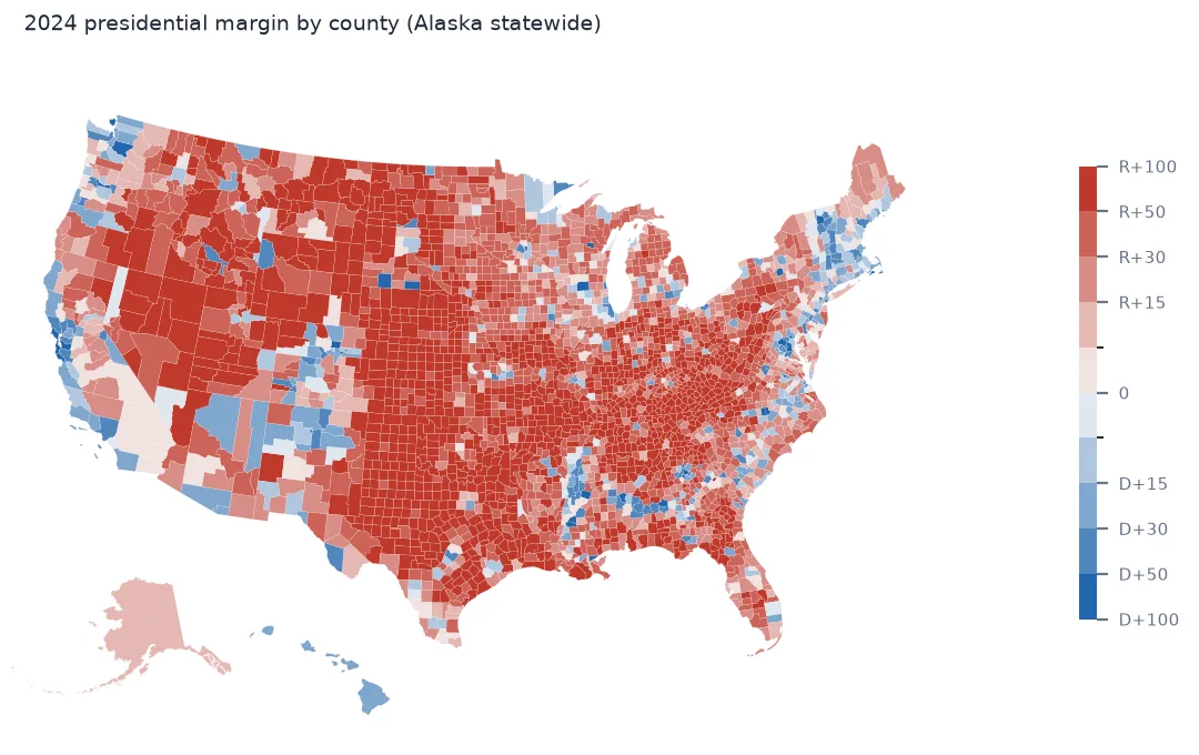
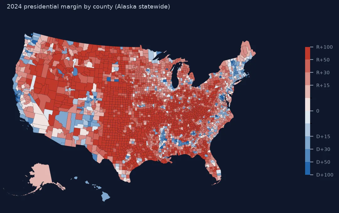
Join, count failures, find hidden collisions, compute the margin

1. Join naively and count what fails

Read the FIPS codes as strings — as integers, Alabama's 01001 becomes 1001 and nothing in the first nine states joins — and look at both sides of an outer join:

naive = counties.merge(results, left_on="GEOID", right_on="county_fips", how="outer", indicator=True)
print(naive._merge.value_counts().to_dict())
print("results without a shape:", naive[naive._merge == "right_only"].state_name.value_counts().to_dict())
print("shapes without a result:", naive[naive._merge == "left_only"].STUSPS.value_counts().to_dict())

{'both': 3116, 'right_only': 44, 'left_only': 28}
results without a shape: {'Alaska': 37, 'District of Columbia': 7}
shapes without a result: {'AK': 27, 'HI': 1}

2. Find the collisions the join did not report

Unmatched rows are the easy part. The dangerous rows are the ones that matched wrongly, where a code means one thing in the results and another in the boundaries:

dc = results[results.state_name == "District of Columbia"]
print(f"DC: {len(dc)} rows, codes {dc.county_fips.min()}-{dc.county_fips.max()}; "
      f"ward 1 alone is {dc.total_votes.iloc[0]:,} of {dc.total_votes.sum():,} votes")
ak = naive[(naive._merge == "both") & (naive.STUSPS == "AK")]
print("Alaska codes that 'matched':", [(r.GEOID, r.NAME, r.county_name) for r in ak.itertuples()])

DC: 8 rows, codes 11001-11008; ward 1 alone is 40,463 of 325,869 votes
Alaska codes that 'matched': [('02013', 'Aleutians East', 'State House District 13'), ('02016', 'Aleutians West', 'State House District 16'), ('02020', 'Anchorage', 'State House District 20')]

DC's first ward carries the county code 11001, so a naive join paints all of Washington with one ward's result. Alaska's results come by state house district, numbered 02001–02040, and three of those numbers happen to be borough codes. One is Anchorage's 02020, which silently receives house district 20's votes. There is no county-level presidential result for Alaska, so the honest map shows the state as one unit.

3. Compute the margin, not the winner

A winner-take-all map colours a county that went 50.1% exactly like one that went 90%. The margin — the Republican share minus the Democratic share, as a fraction of all votes — keeps that information:

print(gdf.margin.describe().round(3).to_string())
bins = [-1, -0.3, -0.1, 0, 0.1, 0.3, 1]
print(pd.cut(gdf.margin, bins).value_counts().sort_index().to_string())

count    3114.000
mean        0.352
std         0.313
min        -0.838
25%         0.174
50%         0.420
75%         0.596
max         0.925
margin
(-1.0, -0.3]     128
(-0.3, -0.1]     196
(-0.1, 0.0]      128
(0.0, 0.1]       175
(0.1, 0.3]       513
(0.3, 1.0]      1974

Nearly two thirds of counties, 1,974 of 3,114, went Republican by 30 points or more. A winner map hides that, along with the 303 counties decided by less than 10 points.

4. Project, and inset Alaska and Hawaii

Draw the contiguous states in an equal-area projection (Albers, EPSG:5070) so county areas are comparable, and Alaska and Hawaii in their own projections on separate axes:

fig = plt.figure(figsize=(9, 5.6))
main, ak_ax, hi_ax = fig.add_axes([0, 0.08, 0.86, 0.86]), fig.add_axes([0, 0, 0.22, 0.3]), fig.add_axes([0.22, 0, 0.14, 0.2])
for ax, part, crs in ((main, ~gdf.STATEFP.isin(["02", "15"]), 5070), (ak_ax, gdf.STATEFP == "02", 3338), (hi_ax, gdf.STATEFP == "15", 32604)):
    gdf[part & gdf.margin.notna()].to_crs(crs).plot(ax=ax, column="margin", cmap="RdBu_r", vmin=-0.6, vmax=0.6, linewidth=0)
    ax.set_axis_off()
fig.savefig("data/county_margin_2024.png", dpi=150)
print("saved", Path("data/county_margin_2024.png").stat().st_size // 1000, "kB")

saved 394 kB

5. Measure what the map exaggerates

g = gdf.dropna(subset=["margin"]).to_crs(5070)
g["km2"] = g.area / 1e6
r = g.margin > 0
print(f"Republican-won counties: {r.sum():,} of {len(g):,}, {g.km2[r].sum() / g.km2.sum():.0%} of the land, "
      f"{g.total_votes[r].sum() / g.total_votes.sum():.0%} of the votes")
print(f"national two-party picture: R {g.votes_gop.sum() / g.total_votes.sum():.1%}, D {g.votes_dem.sum() / g.total_votes.sum():.1%}")

Republican-won counties: 2,662 of 3,114, 88% of the land, 51% of the votes
national two-party picture: R 49.9%, D 48.4%

The map is mostly red because most of the land voted Republican. It does not show that Republican-won counties cast only about half the votes. Large, thinly populated counties dominate the picture. The fixes are cartograms, dot-density maps and value-by-alpha shading, each covered on its own page.

Checking totals and finding the closest counties

The data used on this page

County-level 2024 presidential results compiled from state and county returns in tonmcg/US_County_Level_Election_Results_08-24; county boundaries from the US Census Bureau cartographic boundary files, 2023, 1:20 million.

from pathlib import Path

import geopandas as gpd
import matplotlib
matplotlib.use("Agg")
import matplotlib.pyplot as plt
import numpy as np
import pandas as pd
import requests

Path("data").mkdir(exist_ok=True)
SRC = "https://raw.githubusercontent.com/tonmcg/US_County_Level_Election_Results_08-24/master/"
for name, url in {"2024_US_County_Level_Presidential_Results.csv": SRC + "2024_US_County_Level_Presidential_Results.csv",
                  "cb_2023_us_county_20m.zip": "https://www2.census.gov/geo/tiger/GENZ2023/shp/cb_2023_us_county_20m.zip"}.items():
    if not Path("data", name).exists():
        Path("data", name).write_bytes(requests.get(url, timeout=300).content)
results = pd.read_csv("data/2024_US_County_Level_Presidential_Results.csv", dtype={"county_fips": str})
counties = gpd.read_file("data/cb_2023_us_county_20m.zip")
counties = counties[~counties.STATEFP.isin(["60", "66", "69", "72", "78"])]          # no electoral votes
print(f"{len(results):,} result rows; {len(counties):,} county shapes in the states and DC")

3,160 result rows; 3,144 county shapes in the states and DC

Example 1: check the totals before mapping

print(f"Republican {results.votes_gop.sum():,}  Democratic {results.votes_dem.sum():,}  all {results.total_votes.sum():,}")
print(f"after the fixes: {int(gdf.total_votes.sum()):,} votes mapped, {int(results.total_votes.sum() - gdf.total_votes.sum()):,} not mapped")
print("unmapped:", res[~res.fips.isin(gdf.fips)].fips.tolist(), "| Kalawao (15005) is in the shapes but votes with Maui")

Republican 77,294,799  Democratic 75,006,739  all 154,863,739
after the fixes: 154,863,739 votes mapped, 0 not mapped
unmapped: [] | Kalawao (15005) is in the shapes but votes with Maui

The national sums should land within a fraction of a percent of the certified totals. If they do not, a row has been lost or duplicated before the map was even drawn.

Example 2: the closest counties

close = gdf.dropna(subset=["margin"]).assign(abs_margin=lambda d: d.margin.abs()).nsmallest(6, "abs_margin")
print(close[["NAME", "STUSPS", "votes_gop", "votes_dem", "margin"]].round(4).to_string(index=False))

      NAME STUSPS  votes_gop  votes_dem  margin
    Talbot     MD    11125.0    11119.0  0.0003
     Bucks     PA   198722.0   198431.0  0.0007
Tippecanoe     IN    32783.0    32683.0  0.0015
     Green     WI    10843.0    10903.0 -0.0027
 Oktibbeha     MS     8901.0     8851.0  0.0028
   Haywood     TN     3286.0     3311.0 -0.0038

Two datasets never designed for each other

A county election map joins two datasets that were never designed for each other. Election results follow each state's reporting units: counties, wards, townships or legislative districts. Census boundaries follow the federal county list, which changes over time. Connecticut swapped its eight counties for nine planning regions in the 2022 boundaries, and results compilations followed only from 2024. FIPS codes look like a shared key, but a code is just a five-digit string, and two sources can use the same string for different places.

Once joined correctly, the map tells you where each candidate won, by how much, and which places are competitive. What it cannot show is how many people are behind each colour. Rural counties cover most of the land, and an equal-area map faithfully reproduces that, so the picture is dominated by places with few voters. Read a county map as geography, not as a vote count.

Integer FIPS, Connecticut and Virginia's cities

• FIPS as integers drops leading zeros for Alabama through Connecticut; always dtype=str.
• Connecticut results before 2024 use the eight old counties; join them to 2020-era boundaries.
• Virginia's independent cities are county-equivalents with their own FIPS codes; they are tiny on the map but real units.
• Kalawao County, Hawaii has a shape but no separate result; it votes with Maui.
• Third-party votes are in total_votes but not in either party's column, so margins do not sum to the two-party split.
• Result compilations change as states certify; pin the version you used.

Internal links

• Choropleth maps in GeoPandas — the mapping basics
• Choropleth classification explained — choosing the margin classes
• Join attribute data in GeoPandas — the general join
• Choosing a projected CRS — why Albers for the lower 48

FAQ

How do I join election results to county shapes in Python?

Read both FIPS columns as five-character strings, merge with validate="one_to_one", and handle Alaska (house districts), DC (wards) and Kalawao before joining.

Why does Alaska have no county election map?

Alaska reports presidential results by state house district, not by borough; there is no county-level result to map.

Should I map the winner or the margin?

The margin. A winner map gives a 51% county the same colour as a 90% county.

Why is the US county map so red?

Republican-won counties covered 88% of the land in 2024 but cast about half the votes; the map shows area, not voters.