Crime Hotspot Methods Explained

Problem statement

"Hotspot" has no single definition. An analyst can flag the grid cells with the most crime, the peaks of a kernel density surface, the clusters a Getis-Ord Gi* test calls significant, or the neighbourhoods with the highest rates, and each method draws a different map from the same incidents. They answer different questions: where crime is densest, where it is denser than chance, where it is smoothest to patrol. Choosing among them is a decision with consequences, and the evidence for it can be measured on a city's own data.

This page compares five hotspot methods on Chicago's robberies. Each draws hotspots from 2023's robberies on a common grid of 500-foot cells; each is scored by the share of 2024's robberies its hotspots captured, against the share of the city they cover; and their maps are compared cell by cell.

Quick answer

Put every method on the same grid, flag about 5% of the city with each, and score them all against next year's incidents with the predictive accuracy index:

def score(mask):
    hit, area = C24[mask].sum() / C24.sum(), mask.sum() / INSIDE.sum()
    return hit, area, hit / area

rows = [{"method": name, "2024 captured": f"{h:.1%}", "area": f"{a:.1%}", "PAI": round(p, 2)}
        for name, (h, a, p) in ((n, score(m)) for n, m in MASKS.items())]
print(pd.DataFrame(rows).sort_values("PAI", ascending=False).to_string(index=False))

                    method 2024 captured area  PAI
               cell counts         32.7% 5.0% 6.54
               KDE, 500 ft         28.5% 5.0% 5.71
    Gi* hot cells (FDR 5%)         26.9% 6.7% 4.01
             KDE, 2,000 ft         17.9% 5.0% 3.59
community areas by density         18.9% 6.1% 3.08

The ranking runs from raw to smooth. Cells with the most 2023 robberies captured 32.7% of 2024's in 5% of the city, a PAI of 6.54; a 500-foot kernel density surface 28.5%; Gi* hot cells 26.9% in a slightly larger area; a 2,000-foot surface 17.9%; and the six community areas with the highest 2023 density 18.9% in 6.1% of the city, a PAI of 3.08.

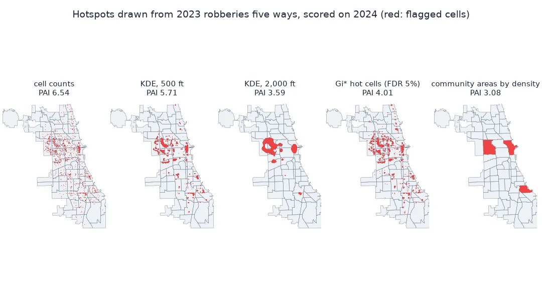
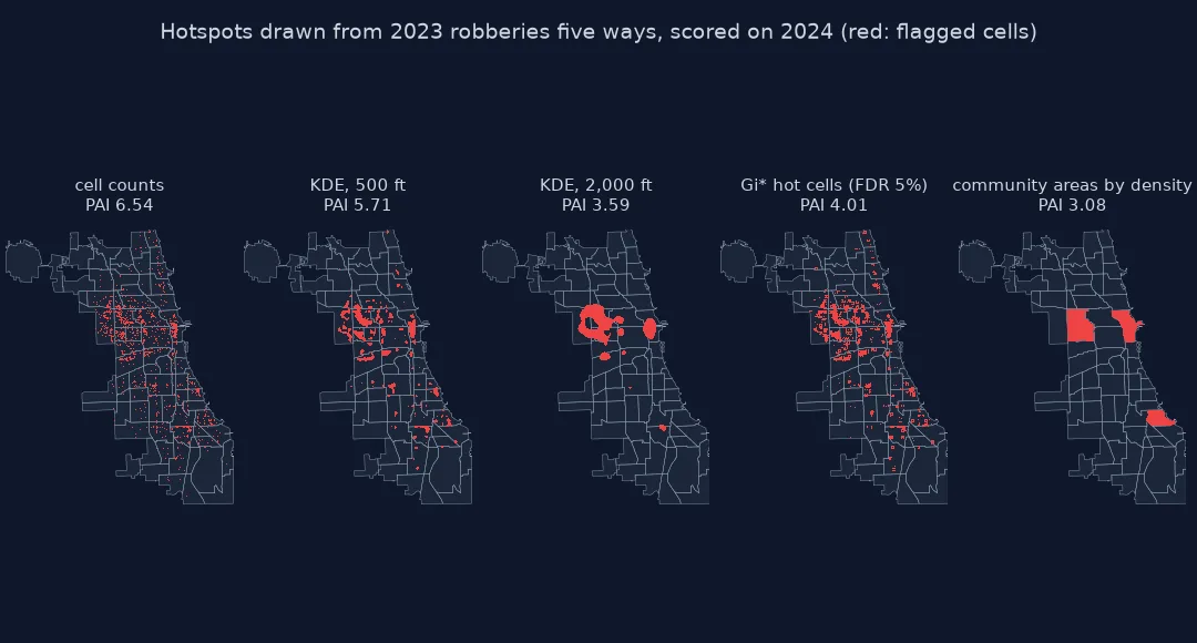
Five methods, their agreement, significance against volume

1. The five methods

All five work from the 2023 robberies and end as a set of 500-foot cells:

for name, m in MASKS.items():
    print(f"{name:28s} {int(m.sum()):>5,} cells flagged")
print(f"cells inside the city: {INSIDE.sum():,}; a 5% target is {int(0.05 * INSIDE.sum()):,} cells")
print(f"community areas chosen by 2023 robbery density: {', '.join(a.title() for a in CHOSEN)}")

cell counts                  1,288 cells flagged
KDE, 500 ft                  1,288 cells flagged
KDE, 2,000 ft                1,288 cells flagged
Gi* hot cells (FDR 5%)       1,727 cells flagged
community areas by density   1,582 cells flagged
cells inside the city: 25,767; a 5% target is 1,288 cells
community areas chosen by 2023 robbery density: West Garfield Park, Loop, Humboldt Park, Near North Side, East Garfield Park, South Shore

The three ranking methods flag exactly 1,288 cells each. Gi* flags 1,727, the cells its test calls significant, and the community-area method 1,582, the cells inside the six densest areas.

2. How much the maps agree

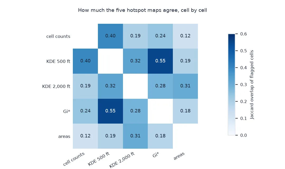
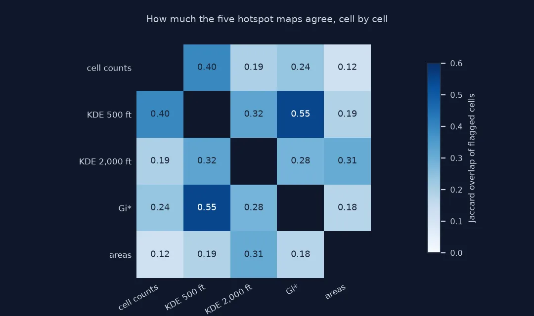
Two hotspot maps can capture similar shares of crime and still flag different places. The Jaccard index, cells flagged by both over cells flagged by either, measures overlap:

names = list(MASKS)
J = pd.DataFrame([[(MASKS[a] & MASKS[b]).sum() / (MASKS[a] | MASKS[b]).sum() for b in names] for a in names], index=names, columns=names)
print(J.round(2).to_string())

                            cell counts  KDE, 500 ft  KDE, 2,000 ft  Gi* hot cells (FDR 5%)  community areas by density
cell counts                        1.00         0.40           0.19                    0.24                        0.12
KDE, 500 ft                        0.40         1.00           0.32                    0.55                        0.19
KDE, 2,000 ft                      0.19         0.32           1.00                    0.28                        0.31
Gi* hot cells (FDR 5%)             0.24         0.55           0.28                    1.00                        0.18
community areas by density         0.12         0.19           0.31                    0.18                        1.00

The closest pair, 500-foot density and Gi*, share 55% of their combined cells; cell counts and community areas share 12%. Methods with similar scores can still point to different places: cell counts and 500-foot density capture similar shares of next year's robberies with only 40% overlap.

3. Why significance is not the same as volume

Gi* flags cells whose neighbourhoods have more robberies than chance, which is not the same as having the most. Compare its flagged cells with the top cells by count:

gi, top = MASKS["Gi* hot cells (FDR 5%)"], MASKS["cell counts"]
print(f"Gi* cells with no 2023 robbery: {(gi & (C23 == 0)).sum()}; top-count cells not flagged by Gi*: {(top & ~gi).sum()}")
print(f"mean 2023 robberies per cell: Gi* {C23[gi].mean():.2f}, top counts {C23[top].mean():.2f}, city {C23[INSIDE].mean():.2f}")

Gi* cells with no 2023 robbery: 573; top-count cells not flagged by Gi*: 707
mean 2023 robberies per cell: Gi* 1.81, top counts 4.08, city 0.43

573 of Gi*'s significant cells had no robbery at all in 2023: they are flagged for their neighbours. And 707 of the 1,288 busiest cells are not flagged: busy cells whose neighbourhoods, taken together, did not pass the test. Gi* cells average 1.81 robberies in 2023, the busiest cells 4.08.

The methods on the year they were fitted to

The data used on this page

The City of Chicago's Crimes - 2001 to Present (ijzp-q8t2), robberies dated 2023 and 2024 with coordinates, projected to EPSG:3435 in US survey feet, and the community area boundaries.

from pathlib import Path

import geopandas as gpd
import numpy as np
import pandas as pd
import requests
import shapely
from esda import fdr
from esda.getisord import G_Local
from libpysal.weights import W
from sklearn.neighbors import KernelDensity

Path("data").mkdir(exist_ok=True)
URL = "https://data.cityofchicago.org/resource/ijzp-q8t2.json"
for year in (2023, 2024):
    f = Path(f"data/robbery_{year}.parquet")
    if not f.exists():
        pd.DataFrame(requests.get(URL, timeout=300, params={"$where": f"year={year} AND primary_type='ROBBERY'", "$limit": 50_000,
                                                           "$order": "id", "$select": "id,date,latitude,longitude"}).json()).to_parquet(f)
G = Path("data/chicago_community_areas.geojson")
if not G.exists():
    G.write_bytes(requests.get("https://data.cityofchicago.org/resource/igwz-8jzy.geojson?$limit=100", timeout=120).content)


def load(year):
    d = pd.read_parquet(f"data/robbery_{year}.parquet").dropna(subset=["latitude", "longitude"]).astype({"latitude": float, "longitude": float})
    return gpd.GeoDataFrame(d, geometry=gpd.points_from_xy(d.longitude, d.latitude), crs=4326).to_crs(3435)


R23, R24 = load(2023), load(2024)
CA = gpd.read_file(G).to_crs(3435)
CITY = CA.union_all()
CELL = 500
X0, Y0, X1, Y1 = CITY.bounds
GX, GY = np.meshgrid(np.arange(X0, X1, CELL) + CELL / 2, np.arange(Y0, Y1, CELL) + CELL / 2)
INSIDE = shapely.contains_xy(CITY, GX, GY)


def counts(p):
    ix = ((p.geometry.x - X0) // CELL).astype(int).to_numpy()
    iy = ((p.geometry.y - Y0) // CELL).astype(int).to_numpy()
    c = np.zeros(GX.shape); np.add.at(c, (iy, ix), 1)
    return c


def kde(bw):
    k = KernelDensity(bandwidth=bw).fit(np.c_[R23.geometry.x, R23.geometry.y])
    return np.where(INSIDE, np.exp(k.score_samples(np.c_[GX.ravel(), GY.ravel()])).reshape(GX.shape), 0)


def top_cells(v, share=0.05):
    flat = np.where(INSIDE, v, -np.inf).ravel()
    m = np.zeros(flat.shape, bool); m[np.argsort(flat)[::-1][:int(share * INSIDE.sum())]] = True
    return m.reshape(GX.shape)


C23, C24 = counts(R23), counts(R24)
K500, K2000 = kde(500), kde(2000)
iy, ix = np.where(INSIDE)
pos = {(a, b): i for i, (a, b) in enumerate(zip(iy, ix))}
w = W({i: [pos[(a + da, b + db)] for da in (-1, 0, 1) for db in (-1, 0, 1) if (da or db) and (a + da, b + db) in pos]
       for (a, b), i in pos.items()}, silence_warnings=True)
g = G_Local(C23[iy, ix], w, star=True, transform="B", permutations=999, seed=1)
hot = (g.Zs > 0) & (g.p_sim <= fdr(g.p_sim, 0.05))
GI = np.zeros(GX.shape, bool); GI[iy[hot], ix[hot]] = True
dens = gpd.sjoin(R23, CA[["community", "geometry"]], predicate="within").groupby("community").size() / CA.set_index("community").area
order = dens.sort_values(ascending=False).index
share = CA.set_index("community").area[order].cumsum() / CA.area.sum()
CHOSEN = list(order[share.shift(fill_value=0) < 0.05])
MASKS = {"cell counts": top_cells(C23 + K500 / K500.max() * 1e-3),      # ties in the count broken by the density
         "KDE, 500 ft": top_cells(K500),
         "KDE, 2,000 ft": top_cells(K2000),
         "Gi* hot cells (FDR 5%)": GI,
         "community areas by density": shapely.contains_xy(CA[CA.community.isin(CHOSEN)].union_all(), GX, GY) & INSIDE}
print(f"robberies with coordinates: {len(R23):,} in 2023, {len(R24):,} in 2024; {INSIDE.sum():,} cells of {CELL} ft")

robberies with coordinates: 11,027 in 2023, 9,085 in 2024; 25,767 cells of 500 ft

Example 1: the same methods, on the year they were fitted to

Scoring a method on its own year flatters the methods that follow the data most closely:

own = {n: C23[m].sum() / C23.sum() / (m.sum() / INSIDE.sum()) for n, m in MASKS.items()}
nxt = {n: score(m)[2] for n, m in MASKS.items()}
print(pd.DataFrame({"PAI on 2023": own, "PAI on 2024": nxt}).round(2).sort_values("PAI on 2024", ascending=False).to_string())

                            PAI on 2023  PAI on 2024
cell counts                        9.53         6.54
KDE, 500 ft                        6.73         5.71
Gi* hot cells (FDR 5%)             4.23         4.01
KDE, 2,000 ft                      4.14         3.59
community areas by density         2.99         3.08

On the year they were built from, cell counts score 9.53; on the next year, 6.54. The drop is largest for cell counts, and the community areas even score slightly better on 2024 than on 2023; but the order at the top holds, and raw counts still lead.

From raw counts to smooth surfaces

The five methods sit on a spectrum from raw to smooth. Cell counts take the data at face value. Kernel density spreads each incident over its neighbourhood, more widely as the bandwidth grows. Gi* asks a different question, whether a cell's neighbourhood has more than chance would give, and answers it with a significance test rather than a ranking. Community areas are the smoothest, averaging over whole neighbourhoods. On Chicago's robberies the raw end predicted the next year best, because robbery returns to the same few blocks; wide smoothing and large areas spread the hotspot over places where little happens.

That ordering is a property of this offence and this city, not a rule. For a rare offence, cell counts are mostly zeros and ones, and some smoothing is needed to find anything stable. For planning patrols, a map of a few contiguous zones may serve better than hundreds of scattered cells, even at a lower PAI. And significance testing has a place where the question is whether a cluster exists at all, not where to send resources.

What carries over is the procedure. Put the methods on a common footing, a shared grid and a comparable share of area; score them on data they were not built from; and look at where they disagree, because a method choice is a choice of which places get attention.

Unequal areas, grid size and ethics

• Unequal areas: Gi* and the community-area method do not flag exactly 5%; PAI divides by the actual area, which keeps them comparable.
• Grid size: 500-foot cells suit block-level robbery; coarser grids favour smoother methods.
• More years: two years make one test; averaging over several pairs of years gives a steadier ranking.
• Other measures: the recapture rate index and hit rates per patrol hour are alternatives to PAI used in policing research.
• Ethics: hotspot maps drawn from recorded crime direct attention to where crime was recorded, which includes where police already were.

Internal links

• How to map crime hotspots with kernel density in Python — the density method and bandwidths
• How to find statistically significant crime hotspots on a hex grid in Python — Gi* in detail
• Crime concentration explained — why places persist

FAQ

What is the best method for crime hotspot mapping?

It depends on the offence and the purpose; test candidates on data they were not built from. For Chicago robbery, 2023 cell counts and narrow kernel density predicted 2024 best.

What is the difference between kernel density and Gi* hotspots?

Kernel density ranks places by smoothed volume; Gi* tests whether a place's neighbourhood has more incidents than chance and flags significant clusters.

How do I compare hotspot maps?

Score each on the same later period with the predictive accuracy index, the share of crime captured divided by the share of area flagged, and measure their overlap with the Jaccard index.

Why do different hotspot methods give different maps?

Because they answer different questions, smooth by different amounts and use different units; on Chicago robbery the overlap between pairs of methods ranges from about a tenth to a half.