Recorded Crime Data Explained

Problem statement

A crime map is a map of records, and a record exists only when an offence passes through a chain of steps: someone notices it, someone reports it or police find it, an officer classifies it, a records system stores it, and an open data extract publishes it, minus whatever is withheld. Each step lets some offences through and stops others, and the steps work differently for different offences and places. Reading recorded crime as a measure of how much crime happens, rather than of how much is recorded, is the most common way crime maps mislead.

This page traces that chain through Chicago's data. It separates offences that are recorded almost only when police find them from those reported by victims, measures how their share varies between neighbourhoods and how differently the two groups have moved since 2015, and counts what the publication step removes or blurs.

Quick answer

Find the offence types recorded almost only with an arrest, which mostly come to light through police activity, and see how unevenly they are spread:

by_type = C.groupby("primary_type").arrest.agg(["mean", "size"])
FOUND = by_type[(by_type["mean"] > 0.5) & (by_type["size"] >= 100)].index
C["police_found"] = C.primary_type.isin(FOUND)
share = J.assign(f=J.primary_type.isin(FOUND)).groupby("community").f.mean()
print("recorded mostly with an arrest:", ", ".join(t.lower() for t in FOUND))
print(f"share of all 2024 incidents: {C.police_found.mean():.1%}; by community area {share.min():.1%} to {share.max():.1%}")

recorded mostly with an arrest: concealed carry license violation, interference with public officer, liquor law violation, narcotics, prostitution, weapons violation
share of all 2024 incidents: 5.9%; by community area 0.4% to 20.8%

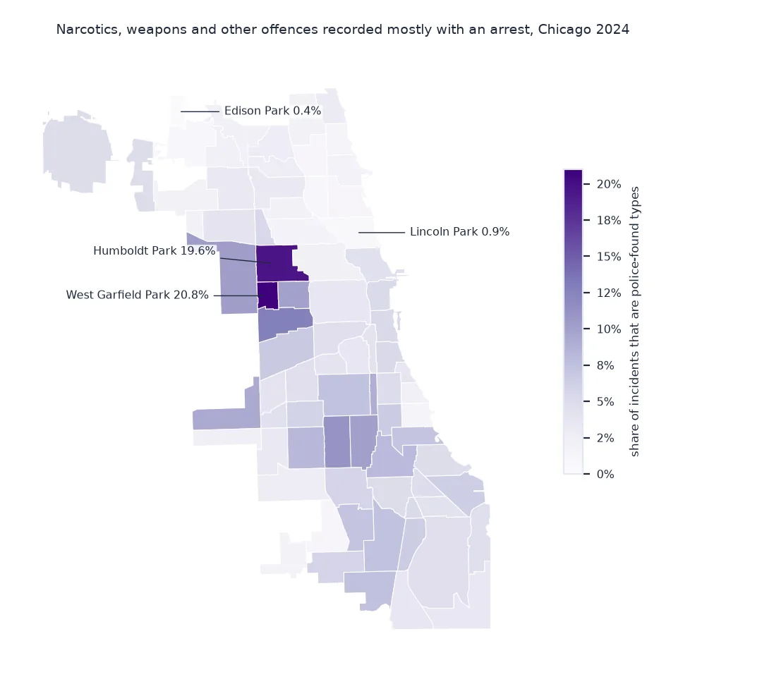
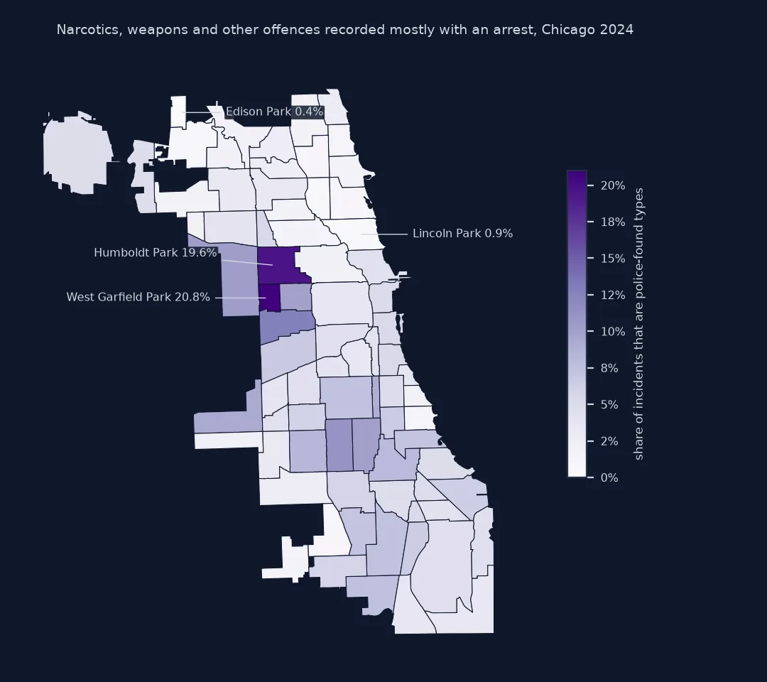
Six offence types end in an arrest more than half the time, from weapons violations at 61% to concealed carry licence violations at 98%. Together they are 5.9% of the city's incidents, but 20.8% in the area where they are most common and 0.4% where they are least: a fifty-fold range, set as much by where police look as by where the offences happen.

Reported against detected, what publication removes

1. Compare the two kinds over time

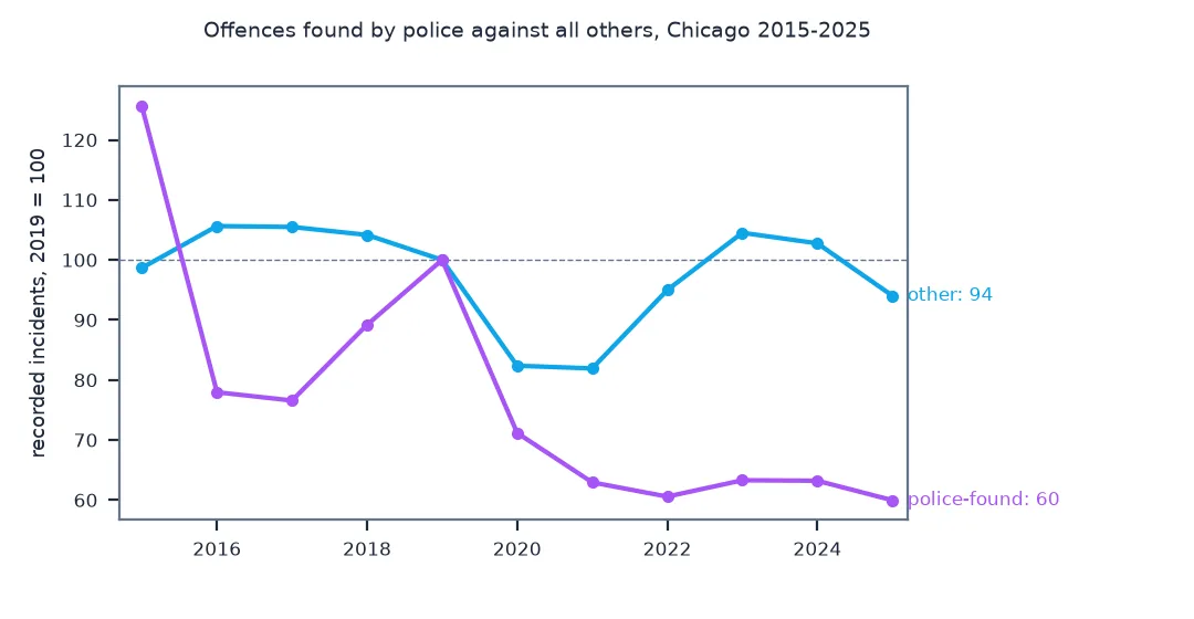
A change in police activity moves the first group directly. Compare yearly counts since 2015, indexed to 2019:

Y["group"] = np.where(Y.primary_type.isin(FOUND), "police-found", "other")
T = Y.pivot_table(index="year", columns="group", values="n", aggfunc="sum")
print((T / T.loc[2019]).round(2).loc[[2015, 2016, 2019, 2021, 2023, 2025]].to_string())
print(f"police-found, 2015 to 2016: {T.loc[2016, 'police-found'] / T.loc[2015, 'police-found'] - 1:+.0%}")

group  other  police-found
year                      
2015    0.99          1.26
2016    1.06          0.78
2019    1.00          1.00
2021    0.82          0.63
2023    1.05          0.63
2025    0.94          0.60
police-found, 2015 to 2016: -38%

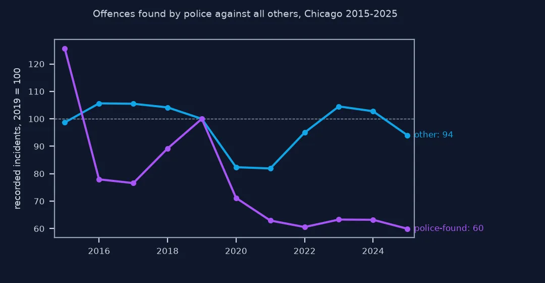
Between 2015 and 2016 the police-found offences fell by 38% while the rest rose by 7%, and by 2025 they stood at 60% of their 2019 level against 94% for everything else. No change in drug use or gun carrying moves that fast; a change in enforcement can.

2. Count what publication removes or blurs

no_xy = C.latitude.isna()
mid1 = (C.time.dt.day == 1) & (C.time.dt.hour == 0) & (C.time.dt.minute == 0)
xy = C.latitude.astype(str) + C.longitude.astype(str)
print(f"published without a location: {no_xy.mean():.1%}")
print(f"dated by placeholder (00:00 on the 1st): {mid1.mean():.1%}")
print(f"sharing exact coordinates with another incident (block-level points): {xy[~no_xy].duplicated(keep=False).mean():.1%}")

published without a location: 0.8%
dated by placeholder (00:00 on the 1st): 0.4%
sharing exact coordinates with another incident (block-level points): 67.9%

0.8% of records are published without a location and 0.4% carry a placeholder date. Two thirds share their exact coordinates with another incident, because locations are moved to a few points per block.

3. See which offences arrive by report after the fact

Offences reported long after they happen carry vaguer dates. The share of each type timed exactly at midnight is a rough marker:

midnight = (C.time.dt.hour == 0) & (C.time.dt.minute == 0)
m = C.assign(m=midnight).groupby("primary_type").m.agg(["mean", "size"])
m = m[m["size"] >= 1000].sort_values("mean", ascending=False)
print(m["mean"].head(4).map("{:.1%}".format).to_string())
print(f"robbery: {m.loc['ROBBERY', 'mean']:.1%}; all incidents: {midnight.mean():.1%}")

primary_type
OFFENSE INVOLVING CHILDREN    19.5%
CRIMINAL SEXUAL ASSAULT       16.8%
SEX OFFENSE                   12.5%
DECEPTIVE PRACTICE            12.5%
robbery: 1.2%; all incidents: 3.6%

Offences involving children and sexual offences, often reported long after they happen, are timed at exactly midnight ten to sixteen times as often as robbery, which is usually reported at once.

The same city, two maps

The data used on this page

The City of Chicago's Crimes - 2001 to Present (ijzp-q8t2): every incident dated 2024, and yearly counts by offence type for 2015–2025 aggregated on the server; and the community area boundaries.

from pathlib import Path

import geopandas as gpd
import numpy as np
import pandas as pd
import requests

Path("data").mkdir(exist_ok=True)
URL = "https://data.cityofchicago.org/resource/ijzp-q8t2.json"
F = Path("data/chicago_crimes_2024.parquet")
if not F.exists():
    rows, offset = [], 0
    while True:
        part = requests.get(URL, timeout=300, params={
            "$where": "year=2024", "$limit": 50_000, "$offset": offset, "$order": "id",
            "$select": "id,date,primary_type,arrest,domestic,community_area,latitude,longitude,location_description,block,updated_on"}).json()
        rows += part; offset += len(part)
        if len(part) < 50_000:
            break
    pd.DataFrame(rows).to_parquet(F)
f = Path("data/yearly_by_type.json")
if not f.exists():
    f.write_bytes(requests.get(URL, timeout=300, params={"$select": "year, primary_type, count(*) AS n",
                                                       "$where": "year BETWEEN 2015 AND 2025", "$group": "year, primary_type",
                                                       "$limit": 5000}).content)
Y = pd.read_json(f).astype({"n": int, "year": int})
G = Path("data/chicago_community_areas.geojson")
if not G.exists():
    G.write_bytes(requests.get("https://data.cityofchicago.org/resource/igwz-8jzy.geojson?$limit=100", timeout=120).content)
C = pd.read_parquet(F).assign(arrest=lambda d: d.arrest.astype(bool))
C["time"] = pd.to_datetime(C.date)
p = C.dropna(subset=["latitude", "longitude"])
p = gpd.GeoDataFrame(p, geometry=gpd.points_from_xy(p.longitude.astype(float), p.latitude.astype(float)), crs=4326)
CA = gpd.read_file(G)
J = gpd.sjoin(p, CA[["community", "geometry"]], predicate="within")
print(f"{len(C):,} incidents in 2024; {Y.year.nunique()} years of counts by type")

259,638 incidents in 2024; 11 years of counts by type

Example 1: the same city, two maps

Rank community areas by all incidents and by incidents excluding the police-found types, and see how much the ranking moves:

counts = J.groupby("community").size()
victim = J[~J.primary_type.isin(FOUND)].groupby("community").size()
moved = (counts.rank(ascending=False) - victim.rank(ascending=False)).abs()
print(f"rank correlation: {counts.corr(victim, method='spearman'):.3f}; largest move {moved.max():.0f} places ({moved.idxmax().title()})")
print(f"Humboldt Park police-found share {share['HUMBOLDT PARK']:.1%}; Lincoln Park {share['LINCOLN PARK']:.1%}")

rank correlation: 0.998; largest move 4 places (Pullman)
Humboldt Park police-found share 19.6%; Lincoln Park 0.9%

Removing the police-found types barely changes the ranking of areas by total incidents, a rank correlation of 0.998, because they are a small share of the total. Their effect is on maps of those offences themselves, and on any measure, such as arrest rates, that they dominate.

The dark figure of crime

Criminologists distinguish the "dark figure" of crime, offences that never reach a record, from recorded crime. How large it is depends on the offence. Homicides and car thefts, which usually need a police report for insurance, are among the most fully recorded; minor thefts, many assaults and most frauds are not reported at all in a large share of cases, as victim surveys repeatedly find. A map of recorded theft is partly a map of willingness and means to report.

Offences without a victim to report them work the other way. Drug possession, weapons carrying, prostitution and liquor law violations become records mostly when police find them, which is why nearly every one ends in an arrest. Their geography and their trend follow where and how intensively police look: in Chicago they vary fifty-fold between neighbourhoods and fell by 40% between 2019 and 2025 while other offences fell by 6%. That is not evidence that drug use fell or that it is concentrated where the records are.

The publication step adds its own layer: locations moved to the block, some withheld, dates defaulted when unknown, records arriving and changing after the fact, and from October 2025 coordinates removed almost entirely. None of this makes recorded crime useless. It makes the record, not the offence, the unit of analysis, and it means every map should say which offences it shows and why.

Victim surveys, calls for service and feedback

• Victim surveys: national surveys such as the US National Crime Victimization Survey estimate reporting rates by offence; they are not available for single neighbourhoods.
• Calls for service: 911 call data records demand rather than offences, with its own biases; it complements incident data.
• Classification: the line between assault and battery, or theft and burglary, depends on facts an officer records at the time and may revise.
• Domestic incidents: the domestic flag marks a large share of batteries; their reporting depends strongly on circumstances.
• Feedback: patrols sent where records are high produce more records there, for police-found offences especially.

Internal links

• How to download and map city crime data in Python — the dataset and its description
• How to compare arrest rates between areas in Python — the offence mix and arrests
• Why do my crime counts change every time I download the data? — records that keep changing

FAQ

What does recorded crime data measure?

Offences that were reported to or found by police, classified and entered into a records system, and published; not all offences that happened.

Why do drug offences cluster where police patrol?

Because they are recorded mostly when police find them; in Chicago nearly every narcotics incident ends in an arrest, and their geography follows enforcement.

What is the dark figure of crime?

The offences that never become records, because they are not noticed, not reported, or not recorded; its size varies greatly by offence type.

Can recorded crime show crime trends?

For offences reported reliably, such as homicide and car theft, reasonably well; for offences found mainly by police, trends follow enforcement as much as offending.