
Why Does My Crime Rate for a Small Area Change So Much?
On this page
Problem statement
You compute crime rates by neighbourhood for two years and the smallest neighbourhood's rate has doubled, or halved, while the large ones barely moved. Next year's map will show it somewhere else again. Two things are happening. A small population means a small count, and a small count moves a long way by chance. And a small area, especially a long and narrow one, has a large share of its incidents near its edges, so the count itself depends on how incidents are assigned to areas: by a recorded area code or by a spatial join.
This page measures both for robbery in Chicago's 77 community areas in 2023 and 2024: how much rates change from one year to the next by population size, how far counts from the recorded area field and from a spatial join disagree, and what pooling years and empirical Bayes smoothing do to the smallest area, Fuller Park, with about 2,200 residents.
Quick answer
Compare the year-to-year change in rates by population size before reading anything into a small area's change:
T["size"] = pd.qcut(T.residents, 3, labels=["smallest third", "middle third", "largest third"])
T["change"] = T.rate_2024 / T.rate_2023 - 1
print(T.groupby("size", observed=True).change.apply(lambda c: c.abs().median()).map("{:.0%}".format).rename("median change, 2023 to 2024").to_string())
fp = T.loc["FULLER PARK"]
print(f"Fuller Park, {fp.residents:,.0f} residents: {fp.field_2023:.0f} robberies in 2023, {fp.field_2024:.0f} in 2024; "
      f"rate {fp.rate_2023:.0f} -> {fp.rate_2024:.0f} per 10,000")
size
smallest third 24%
middle third 19%
largest third 16%
Fuller Park, 2,186 residents: 31 robberies in 2023, 63 in 2024; rate 142 -> 288 per 10,000
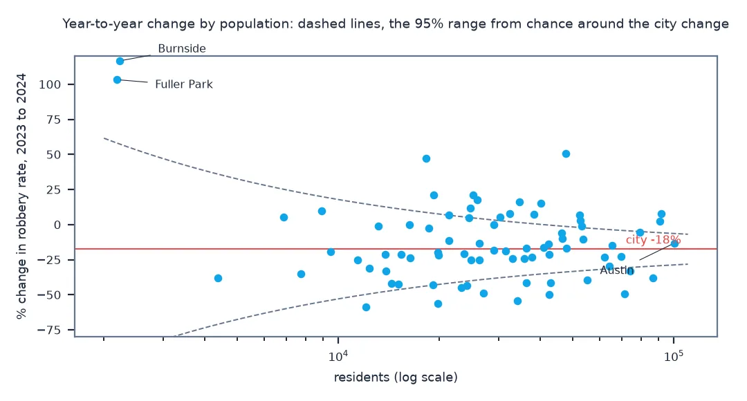
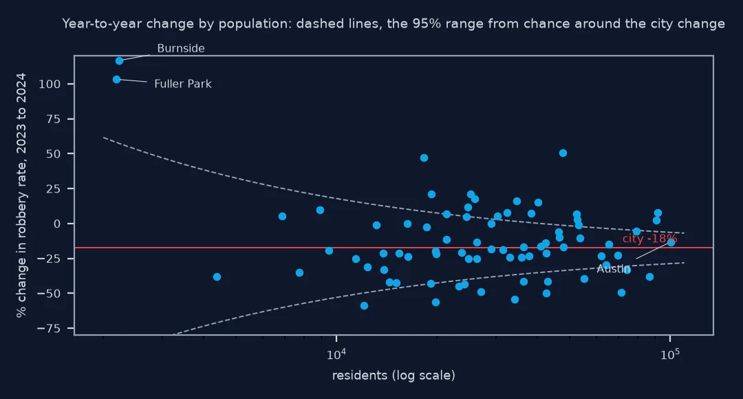
Rates in the smallest third of areas changed by a median 24% between the two years, against 16% in the largest third. Fuller Park's doubled, from 31 robberies to 63, which moved its rate from 142 to 288 per 10,000 and from second to first in the city.
Recorded areas against joins, pooled years, empirical Bayes
1. Compare the recorded area with a spatial join
Each record carries a community area code; the point can also be joined to the boundaries. The two disagree for a few percent of records, and the disagreement is not spread evenly:
T["gap_2024"] = T.spatial_2024 / T.field_2024 - 1
print(f"records where field and join disagree, 2024: {DISAGREE:.1%}")
print(T.reindex(T.gap_2024.abs().sort_values(ascending=False).index)[["residents", "field_2024", "spatial_2024", "gap_2024"]].head(4).round(2).to_string())
print(f"rank correlation of |gap| with area size (sq mi): {T.gap_2024.abs().corr(T.sq_mi, method='spearman'):.2f}")
fp = CA[CA.community == "FULLER PARK"]
p24 = pts[(pts.year == 2024) & (pts.community_area == fp.area_numbe.iloc[0])]
out = p24[~p24.within(fp.geometry.iloc[0])]
print(f"Fuller Park robberies whose point is outside it: {len(out)}; distance from the boundary: at most {out.distance(fp.geometry.iloc[0].boundary).max():.1f} ft")
records where field and join disagree, 2024: 3.3%
residents field_2024 spatial_2024 gap_2024
community
FULLER PARK 2186.0 63 44 -0.30
BEVERLY 19811.0 14 18 0.29
MONTCLARE 13755.0 11 14 0.27
DUNNING 42548.0 26 20 -0.23
rank correlation of |gap| with area size (sq mi): -0.32
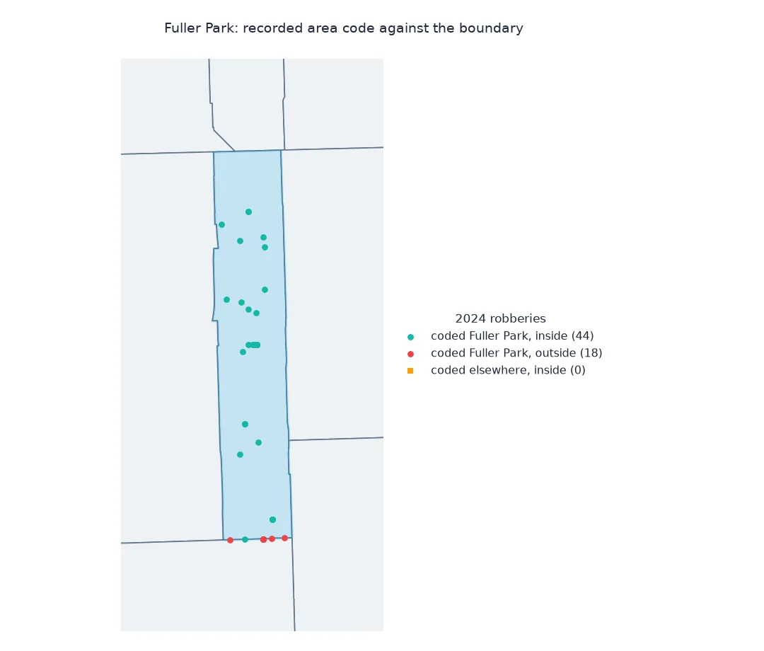
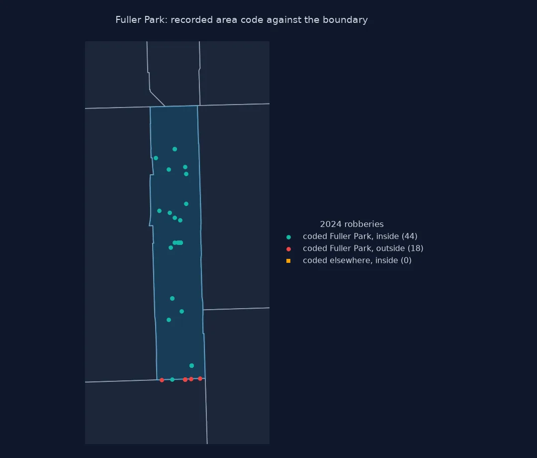
Fuller Park robberies whose point is outside it: 18; distance from the boundary: at most 0.5 ft
3.3% of 2024's robberies carry an area code that differs from the area their point falls in. For Fuller Park the two counts are 63 and 44, a gap of 30%. All 18 of its coded robberies that fall outside it lie within half a foot of its boundary: they are on the boundary street itself, whose centreline is the line between two areas, and the area code records which side the officer chose. Smaller areas tend to have larger gaps, with a rank correlation of -0.32 between the gap and the area's size.
2. Pool years
Two years of robberies over two years of population halves the variance of a Poisson count's rate:
T["rate_pooled"] = (T.field_2023 + T.field_2024) / 2 / T.residents * 1e4
print(T.sort_values("rate_pooled", ascending=False)[["residents", "rate_2023", "rate_2024", "rate_pooled"]].head(4).round(1).to_string())
residents rate_2023 rate_2024 rate_pooled
community
FULLER PARK 2186.0 141.8 288.2 215.0
WEST GARFIELD PARK 16345.0 143.2 109.5 126.3
CHATHAM 31440.0 113.5 92.2 102.9
EAST GARFIELD PARK 19855.0 113.8 89.1 101.5
Pooled over two years, Fuller Park's rate is 215, between its two single-year values, and still the highest; West Garfield Park, which led in 2023, is second.
3. Smooth with empirical Bayes
Empirical Bayes pulls each area's rate towards the city-wide rate, more strongly the smaller its population:
eb = Empirical_Bayes(T.field_2024.values.reshape(-1, 1), T.residents.values.reshape(-1, 1))
T["rate_eb"] = eb.r.flatten() * 1e4
T["shrink"] = 1 - (T.rate_eb - CITY) / (T.rate_2024 - CITY)
print(f"city rate 2024: {CITY:.1f} per 10,000")
print(T.loc[["FULLER PARK", "BURNSIDE", "OAKLAND", "AUSTIN"], ["residents", "field_2024", "rate_2024", "rate_eb", "shrink"]].round(2).to_string())
city rate 2024: 34.4 per 10,000
residents field_2024 rate_2024 rate_eb shrink
community
FULLER PARK 2186.0 63 288.20 238.06 0.20
BURNSIDE 2229.0 13 58.32 53.67 0.19
OAKLAND 4373.0 23 52.60 50.60 0.11
AUSTIN 100278.0 625 62.33 62.18 0.01
Smoothing moves Fuller Park from 288 to 238 per 10,000, a fifth of the way towards the city's 34.4, and Austin, with 100,278 residents, by 1%. With 63 robberies, Fuller Park's count is large enough that the method trusts most of it.
How much each area is shrunk
The data used on this page
The City of Chicago's Crimes - 2001 to Present (ijzp-q8t2), robberies dated 2023 and 2024 with their recorded community area and coordinates; the city's ACS 5 Year Data by Community Area for 2019–2023 populations; and the community area boundaries.
from pathlib import Path

import geopandas as gpd
import numpy as np
import pandas as pd
import requests
from esda.smoothing import Empirical_Bayes

Path("data").mkdir(exist_ok=True)
URL = "https://data.cityofchicago.org/resource/ijzp-q8t2.json"
F = Path("data/robbery_2023_2024.parquet")
if not F.exists():
    pd.DataFrame(requests.get(URL, timeout=300, params={
        "$where": "primary_type = 'ROBBERY' AND year IN (2023, 2024)", "$limit": 50_000,
        "$select": "id, year, community_area, latitude, longitude"}).json()).to_parquet(F)
R = pd.read_parquet(F).dropna(subset=["community_area"]).astype({"year": int, "community_area": int})
R = R[R.community_area > 0]
G = Path("data/chicago_community_areas.geojson")
if not G.exists():
    G.write_bytes(requests.get("https://data.cityofchicago.org/resource/igwz-8jzy.geojson?$limit=100", timeout=120).content)
CA = gpd.read_file(G).astype({"area_numbe": int}).to_crs(3435)
acs = pd.DataFrame(requests.get("https://data.cityofchicago.org/resource/t68z-cikk.json", timeout=120, params={"acs_year": "2023", "$limit": 200}).json())
CA["residents"] = CA.community.map(acs.set_index("community_area").total_population.astype(float))
CA["sq_mi"] = CA.area / 5280 ** 2

pts = R.dropna(subset=["latitude", "longitude"])
pts = gpd.GeoDataFrame(pts, geometry=gpd.points_from_xy(pts.longitude.astype(float), pts.latitude.astype(float)), crs=4326).to_crs(3435)
j = gpd.sjoin(pts, CA[["area_numbe", "geometry"]], predicate="within")
DISAGREE = (j[j.year == 2024].community_area != j[j.year == 2024].area_numbe).mean()
T = CA.set_index("area_numbe")[["community", "residents", "sq_mi"]]
for y in (2023, 2024):
    T[f"field_{y}"] = R[R.year == y].groupby("community_area").size().reindex(T.index, fill_value=0)
    T[f"spatial_{y}"] = j[j.year == y].groupby("area_numbe").size().reindex(T.index, fill_value=0)
    T[f"rate_{y}"] = T[f"field_{y}"] / T.residents * 1e4
T = T.set_index("community")
CITY = T.field_2024.sum() / T.residents.sum() * 1e4
print(f"{len(R):,} robberies with an area code; {len(T)} areas, {T.residents.min():,.0f} to {T.residents.max():,.0f} residents")
20,160 robberies with an area code; 77 areas, 2,186 to 100,278 residents
Example 1: how much each area is shrunk
The shrinkage depends on population, and on how far the rate is from the city's:
w = T[(T.rate_2024 - CITY).abs() > 5]
print(f"rank correlation of shrinkage with population: {w.shrink.corr(w.residents, method='spearman'):.2f}")
print(f"areas under 10,000 residents: median shrinkage {w[w.residents < 10_000].shrink.median():.0%}; "
      f"over 50,000: {w[w.residents > 50_000].shrink.median():.0%}")
print(f"largest change in rank from smoothing: {(T.rate_2024.rank(ascending=False) - T.rate_eb.rank(ascending=False)).abs().max():.0f} places")
rank correlation of shrinkage with population: -1.00
areas under 10,000 residents: median shrinkage 9%; over 50,000: 1%
largest change in rank from smoothing: 1 places
Shrinkage falls with population, perfectly in rank order, from a median 9% for areas under 10,000 residents to 1% for those over 50,000. No area moves more than one place in the ranking: for an offence as common as robbery, the instability that matters here is from year to year, which smoothing a single year cannot remove.
Rare counts behave like Poisson variables
A rate is a count divided by a population, and for a rare event the count behaves roughly like a Poisson variable: its standard deviation is the square root of its mean. Twenty-five robberies a year will often be 20 or 30; in an area of 2,000 people that moves the rate by 25 per 10,000 either way, while in an area of 50,000 the same swing in count barely registers. Year-to-year changes in small areas are therefore mostly noise, and the top of a single year's rate ranking is crowded with small places.
Small areas also suffer more from how incidents are assigned. A narrow neighbourhood like Fuller Park has much of its activity on its boundary streets, and since a boundary street's centreline is the line between two areas, the recorded area code and a spatial join of centreline points can disagree by a large fraction of its count. Neither method is clearly right; the difference is part of the uncertainty and should be reported as such for small areas.
The fixes all trade detail for stability. Pooling years keeps the geography and loses time; empirical Bayes keeps both but borrows strength from the city-wide rate, pulling small areas towards it in proportion to their uncertainty; and aggregating small areas into larger ones loses the geography. None removes the need to show the count beside the rate.
Spatial smoothing, zero counts and rank maps
- Spatial empirical Bayes: shrinking towards the neighbours' rate instead of the city's keeps local patterns;
esda.smoothing.Spatial_Empirical_Bayestakes a weights object. - Population uncertainty: ACS estimates for small areas have their own margins of error; the denominator is uncertain too.
- Zero counts: an area with no robberies has a rate of zero, which smoothing raises towards the city rate.
- Thresholds: suppressing rates below a minimum count, such as 20, is the simplest rule and common in official statistics.
- Rank maps: ranking areas by rate exaggerates noise; credible intervals or funnel plots show what is distinguishable.
Internal links
- How to smooth unstable area rates with empirical Bayes in Python — the method in detail
- Small numbers explained: why rates in small areas jump around — the statistics
- How to calculate crime rates per resident in Python — rates and denominators
FAQ
Why do crime rates change so much in small neighbourhoods?
Because a small population gives a small count, and small counts vary a lot by chance; in Chicago, robbery rates in the smallest third of community areas changed by a median 24% between 2023 and 2024, against 16% in the largest third.
How do I stabilise crime rates for small areas?
Pool several years, smooth with empirical Bayes, or merge small areas; and always show the count beside the rate.
Should I use the recorded area code or a spatial join to count crimes by area?
Check both: they agree for most records, but in small or narrow areas the difference can be a large share of the count.
What does empirical Bayes smoothing do to crime rates?
It moves each area's rate towards the overall rate, by more for areas with small populations, where the observed rate is least reliable.