Why Are So Many of My Crime Points in Exactly the Same Place?

Problem statement

You plot a year of crime incidents as dots, and the map looks emptier than the numbers say it should. Or a nearest-neighbour statistic comes out as zero. Or a clustering algorithm finds hundreds of "clusters" of identical points. The reason is that crime locations are published at block level: to protect victims, each incident is moved to a point that stands for its block, so every incident on a busy block lands on the same few coordinates. Most incidents are stacked exactly on top of others, and methods that assume each point is a distinct location give wrong answers.

This page measures the stacking in Chicago's 2024 incident data, shows what it does to a dot map and to nearest-neighbour distances, and replaces the stacked dots with counts per location drawn as proportional symbols.

Quick answer

Count incidents per distinct coordinate pair before doing anything that treats points as separate places:

LOC = PTS.groupby(["x", "y"]).size().rename("incidents").reset_index()
stacked = PTS.merge(LOC, on=["x", "y"]).incidents > 1
print(f"{len(PTS):,} incidents at {len(LOC):,} distinct locations; used once: {(LOC.incidents == 1).sum():,}")
print(f"incidents sharing their exact location with another: {stacked.mean():.1%}; most at one point: {LOC.incidents.max()}")

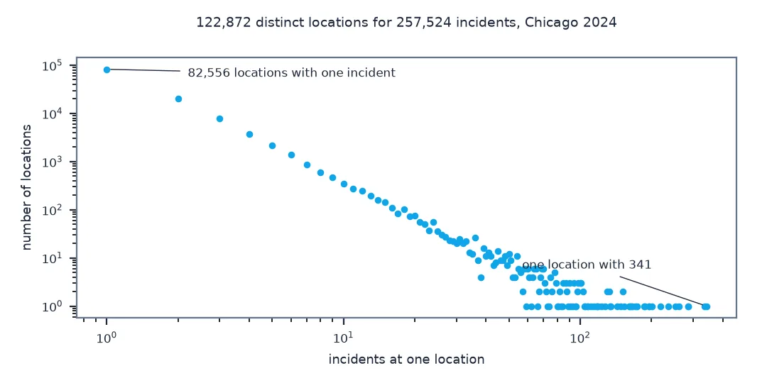
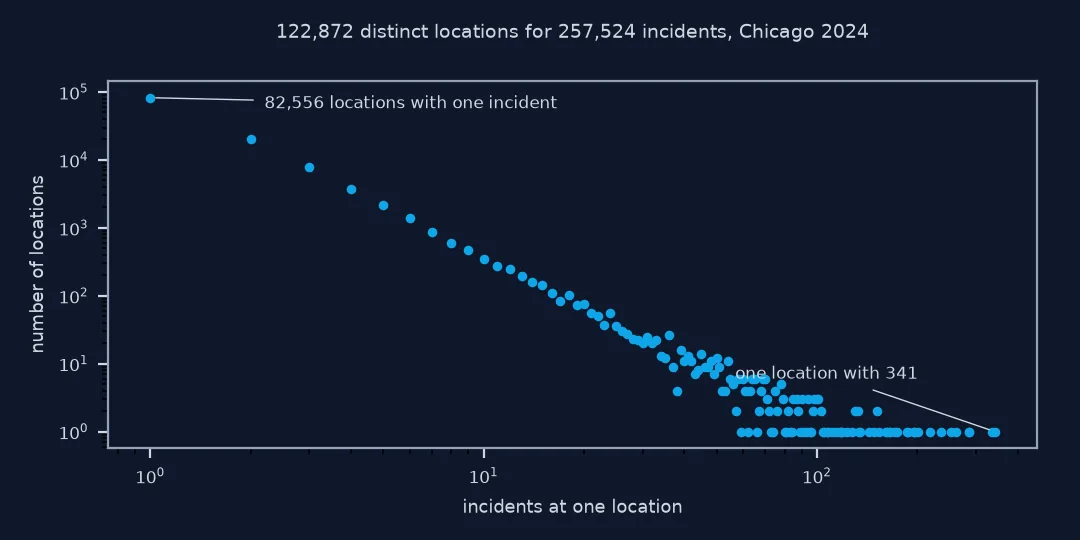
257,524 incidents at 122,872 distinct locations; used once: 82,556
incidents sharing their exact location with another: 67.9%; most at one point: 341

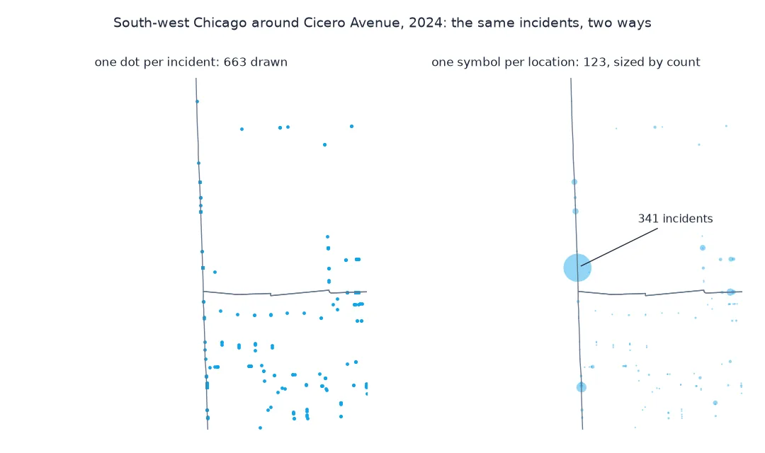
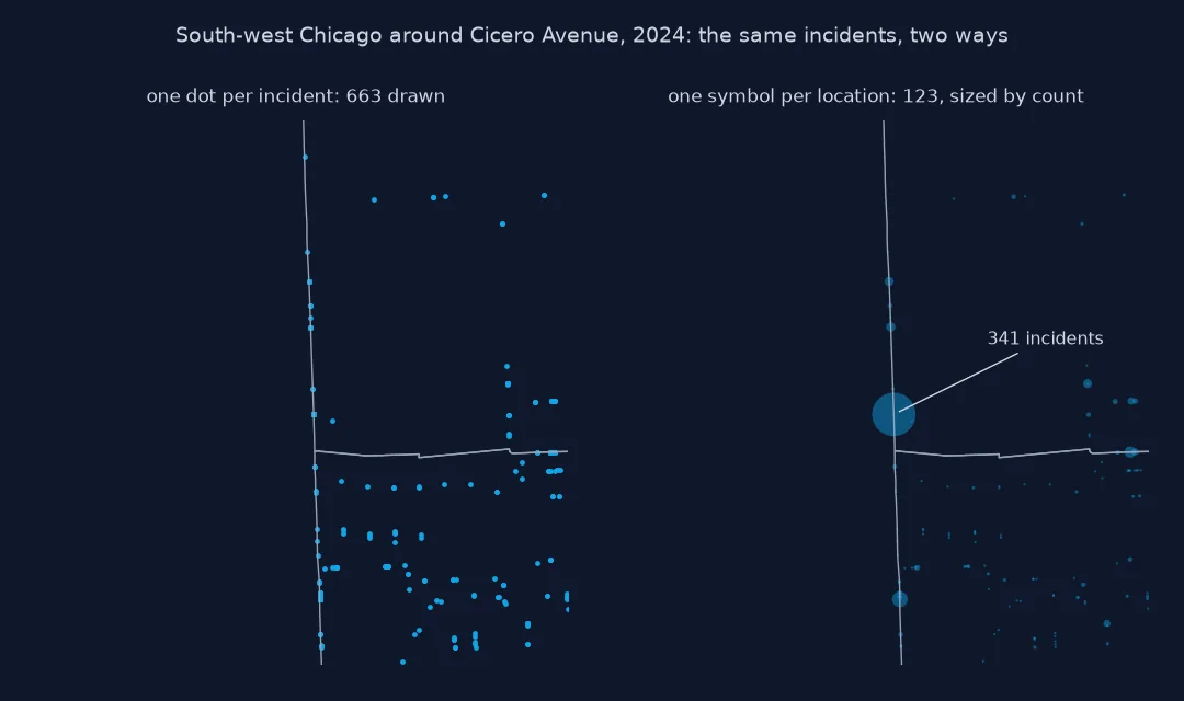
The 257,524 incidents of 2024 occupy 122,872 distinct points. Two thirds of incidents, 67.9%, share their exact coordinates with at least one other; one point on the 7600 block of South Cicero Avenue carries 341.

Effects on nearest-neighbour distances and dot maps

1. See what it does to nearest-neighbour distances

Nearest-neighbour statistics compare each point's distance to its nearest neighbour with what a random pattern would give. With stacked points the nearest neighbour is usually at distance zero:

xy = PTS[["x", "y"]].to_numpy()
d, _ = cKDTree(xy).query(xy, k=2)
print(f"incidents whose nearest neighbour is at distance 0: {(d[:, 1] == 0).mean():.1%}; median distance {np.median(d[:, 1]):.0f} ft")
u = LOC[["x", "y"]].to_numpy()
du, _ = cKDTree(u).query(u, k=2)
print(f"distinct locations only: median nearest-neighbour distance {np.median(du[:, 1]):.0f} ft")

incidents whose nearest neighbour is at distance 0: 67.9%; median distance 0 ft
distinct locations only: median nearest-neighbour distance 17 ft

For 67.9% of incidents the nearest neighbour is at zero distance, so the median is zero and any nearest-neighbour index built on it reports extreme clustering. Among distinct locations the median spacing is 17 feet: the positions Chicago uses along a block.

2. See what it does to a dot map

A dot drawn for each incident hides every incident after the first at the same point. Count how many dots a viewer can actually see:

print(f"dots drawn: {len(PTS):,}; dots visible: {len(LOC):,} ({len(LOC) / len(PTS):.0%})")
heavy = LOC.incidents >= 50
print(f"locations with 50 or more incidents: {heavy.sum()}, holding {LOC.incidents[heavy].sum():,} incidents in {heavy.sum()} visible dots")

dots drawn: 257,524; dots visible: 122,872 (48%)
locations with 50 or more incidents: 206, holding 18,253 incidents in 206 visible dots

Less than half the dots drawn can be seen. The 206 busiest points, with 50 or more incidents each, hold 18,253 incidents and look exactly like 206 single incidents on a dot map.

3. Check how many points a block gets

Chicago uses a few points per block rather than one, so stacking is partial. Count distinct locations per block name:

per_block = PTS.assign(B=PTS.block.str.upper()).groupby("B").apply(lambda g: len(g[["x", "y"]].drop_duplicates()), include_groups=False)
print(f"blocks: {len(per_block):,}; distinct locations per block: median {per_block.median():.0f}, 90th percentile {per_block.quantile(0.9):.0f}")

blocks: 27,199; distinct locations per block: median 4, 90th percentile 9

A typical block name carries four distinct points, and nine in ten carry nine or fewer, so stacking is partial: incidents on a block are spread over a handful of positions, not one.

Proportional symbols per location

The data used on this page

The City of Chicago's Crimes - 2001 to Present (ijzp-q8t2), incidents dated 2024 with coordinates, projected to EPSG:3435 in US survey feet, and the community area boundaries.

from pathlib import Path

import geopandas as gpd
import numpy as np
import pandas as pd
import requests
from scipy.spatial import cKDTree

Path("data").mkdir(exist_ok=True)
URL = "https://data.cityofchicago.org/resource/ijzp-q8t2.json"
F = Path("data/chicago_crimes_2024.parquet")
if not F.exists():
    rows, offset = [], 0
    while True:
        part = requests.get(URL, timeout=300, params={
            "$where": "year=2024", "$limit": 50_000, "$offset": offset, "$order": "id",
            "$select": "id,date,primary_type,arrest,domestic,community_area,latitude,longitude,location_description,block,updated_on"}).json()
        rows += part; offset += len(part)
        if len(part) < 50_000:
            break
    pd.DataFrame(rows).to_parquet(F)
G = Path("data/chicago_community_areas.geojson")
if not G.exists():
    G.write_bytes(requests.get("https://data.cityofchicago.org/resource/igwz-8jzy.geojson?$limit=100", timeout=120).content)
c = pd.read_parquet(F).dropna(subset=["latitude", "longitude"])
xy = gpd.GeoSeries(gpd.points_from_xy(c.longitude.astype(float), c.latitude.astype(float)), crs=4326).to_crs(3435)
PTS = c.assign(x=xy.x.round(2).values, y=xy.y.round(2).values)
CA = gpd.read_file(G).to_crs(3435)
print(f"{len(PTS):,} incidents with coordinates")

257,524 incidents with coordinates

Example 1: proportional symbols per location

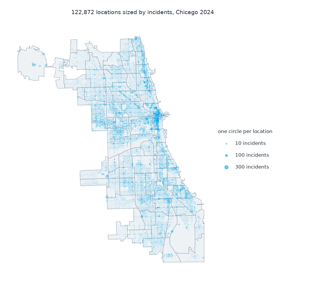
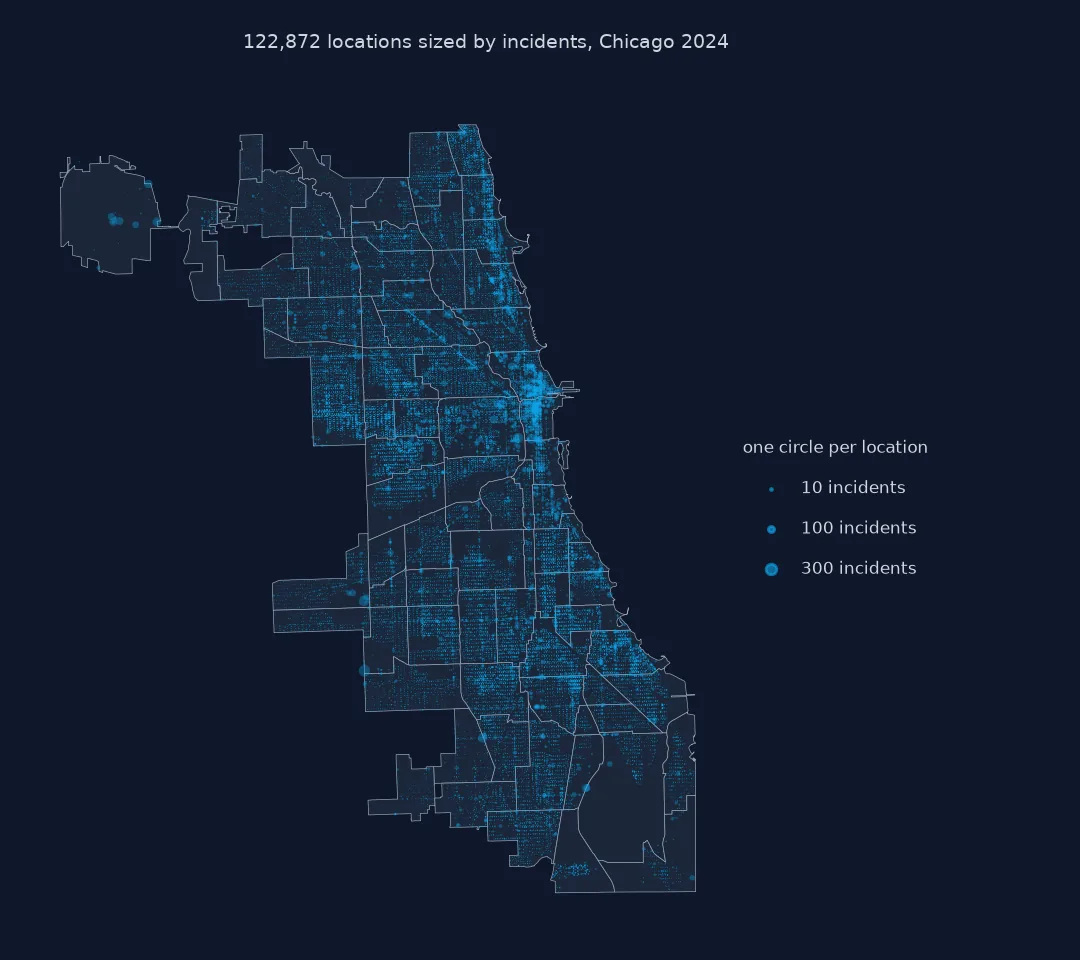
Draw one symbol per distinct location, sized by its count, so the busiest blocks show as the busiest:

import matplotlib
matplotlib.use("Agg")
import matplotlib.pyplot as plt

fig, ax = plt.subplots(figsize=(7, 8))
CA.boundary.plot(ax=ax, color="0.7", linewidth=0.4)
top = LOC.sort_values("incidents")
ax.scatter(top.x, top.y, s=top.incidents / 4, alpha=0.5, linewidths=0)       # area proportional to count
ax.set_axis_off(); fig.savefig("locations.png", dpi=150)
print(f"symbols: {len(top):,}; the largest stands for {top.incidents.max()} incidents, the smallest for 1")

symbols: 122,872; the largest stands for 341 incidents, the smallest for 1

One symbol per location, 122,872 in all, with area proportional to the count, puts the volume back on the map.

Block-level publication protects victims

Block-level publication is a privacy measure. A dataset that gave the exact location of every assault or burglary would identify victims' homes, so police departments move each incident to a point standing for its block or its hundred-block address. In Chicago those points sit on the street centreline, a few per block, and every incident on a block is assigned to one of them. The result is a point pattern made of stacks: 122,872 distinct positions carrying a quarter of a million incidents.

For counting, this does no harm. Counts by area, by street segment, by grid cell or on a kernel density surface come out the same whether the points are stacked or not, because each method adds incidents up. The trouble is with methods that treat each point as a separate place: dot maps, nearest-neighbour distances, Ripley's K at short distances, DBSCAN, and anything that asks how close two incidents were. For those, either work with distinct locations and their counts, or set the shortest distance studied to the size of a block.

Jittering points to spread the stacks is a display device. It makes a dot map show volume, but it invents positions, and analyses run on jittered points measure the jitter. If it is used, say so on the map, and keep the analysis on the published coordinates.

Rounding, boundaries and kernel density

• Rounding: coordinates read from text can differ in the last decimal for the same point; round projected coordinates, here to 0.01 ft, before grouping.
• Boundaries: centreline points on a boundary street sit exactly on the line between two areas; a spatial join can assign them either way.
• Kernel density: unaffected in total, but a bandwidth below the spacing of block points draws the points rather than the pattern.
• Other cities: some publish one point per hundred-block, some an intersection, some a random offset; check the distinct-location count first.
• Do not reverse it: trying to recover exact addresses from block-level data defeats the protection and breaks most portals' terms of use.

Internal links

• How to count crime on street segments in Python — why the points sit on centrelines
• How to test for near-repeat burglary in Python — distance bands that respect the geocoding
• How to map crime hotspots with kernel density in Python — counting methods that are unaffected

FAQ

Why do many crime incidents have identical coordinates?

Because locations are published at block level to protect victims: each incident is moved to a point representing its block, so incidents on the same block share coordinates.

How do I map stacked crime points?

Count incidents per distinct location and draw proportional symbols, or aggregate to segments, cells or areas; a plain dot map hides everything after the first incident at each point.

Can I use nearest-neighbour analysis on crime points?

Not on the raw points: in Chicago's 2024 data most incidents have another at exactly the same place; use distinct locations, or distance bands no shorter than a block.

Should I jitter crime points?

Only for display, and say so; analysis on jittered points measures the jitter, not the crime.