Crime Concentration Explained

Problem statement

One of the most repeated findings in criminology is that crime concentrates in a small share of places: in city after city, about half of recorded crime happens on a few percent of street segments. The finding has a name, the law of crime concentration, and it underpins hot spot policing and place-based prevention. It also hides a statistical trap. When crimes are few and places many, most places have none simply because there are not enough crimes to go round, and the share of places holding half the crime comes out small even if crime were scattered at random.

This page measures concentration on Chicago's 47,057 street segments for all recorded incidents, robbery, burglary and homicide in 2024, compares each with what the same number of crimes scattered at random would give, and tests whether the busiest segments of 2023 were still busy in 2024.

Quick answer

Sort segments by count, find the smallest share holding half the incidents, and compare with a random scattering of the same number:

def share_holding(counts, q=0.5):
    s = np.sort(np.asarray(counts))[::-1]
    return (np.searchsorted(np.cumsum(s) / s.sum(), q) + 1) / len(s)

for t in ("all", "ROBBERY", "BURGLARY", "HOMICIDE"):
    n = SEG[f"n24_{t}"]
    rnd = RNG.poisson(n.sum() / len(n), len(n))                          # same total, no place is special
    print(f"{t.lower():9s} {int(n.sum()):>7,} incidents: half on {share_holding(n):.2%} of segments; at random {share_holding(rnd):.2%}; "
          f"segments with none {(n == 0).mean():.0%}")

all       256,271 incidents: half on 8.78% of segments; at random 34.09%; segments with none 31%
robbery     9,075 incidents: half on 3.20% of segments; at random 8.12%; segments with none 87%
burglary    8,387 incidents: half on 3.94% of segments; at random 7.37%; segments with none 87%
homicide      596 incidents: half on 0.50% of segments; at random 0.64%; segments with none 99%

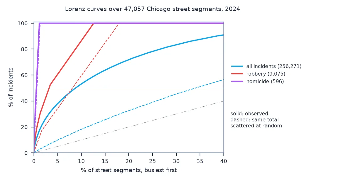
Half of all incidents fell on 8.78% of segments, where a random scattering would need 34.09%: a fourfold concentration beyond chance. For robbery and burglary the gap is about two to one. For homicide it nearly vanishes: half of the 596 fell on 0.50% of segments, and at random they would fall on 0.64%, because with 99% of segments necessarily empty there is almost no room for chance to spread them.

A Lorenz curve, places against areas, persistence

1. Draw the Lorenz curve

The Lorenz curve plots the cumulative share of incidents against the cumulative share of segments, busiest first; the Gini coefficient is twice the area between it and the diagonal:

def gini(counts):
    s = np.sort(np.asarray(counts, dtype=float))
    n = len(s)
    return (2 * np.arange(1, n + 1) - n - 1).dot(s) / (n * s.sum())

for t in ("all", "ROBBERY", "HOMICIDE"):
    n = SEG[f"n24_{t}"]
    print(f"{t.lower():9s} Gini {gini(n):.3f}; for the same total at random {gini(RNG.poisson(n.sum() / len(n), len(n))):.3f}")

all       Gini 0.709; for the same total at random 0.240
robbery   Gini 0.910; for the same total at random 0.842
homicide  Gini 0.990; for the same total at random 0.988

The Gini coefficients say the same. Robbery's 0.910 looks extreme until it is set against 0.842 for random placement; homicide's 0.990 against 0.988 is almost all sparsity.

2. Compare places with areas

Concentration depends on the unit. The same incidents counted in the 77 community areas:

areas = J.groupby("community").size()
print(f"community areas: half of incidents in {share_holding(areas):.0%} of areas; Gini {gini(areas):.3f}")
print(f"street segments: half in {share_holding(SEG.n24_all):.1%} of segments; Gini {gini(SEG.n24_all):.3f}")

community areas: half of incidents in 23% of areas; Gini 0.417
street segments: half in 8.8% of segments; Gini 0.709

Counted in community areas, the same incidents look far more even: half fall in 23% of the 77 areas, with a Gini of 0.417. Large units average busy and quiet places together.

3. Test whether it persists

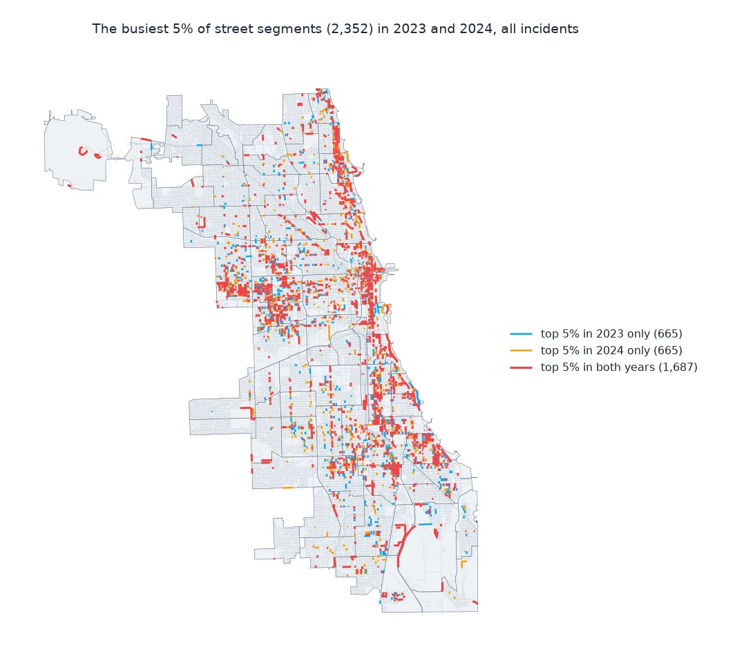
If concentration were chance, the busiest places one year would be ordinary the next. Take the top 5% of segments in 2023 and count their share of 2024:

for t in ("all", "ROBBERY", "BURGLARY", "HOMICIDE"):
    a, b = SEG[f"n24_{t}"], SEG[f"n23_{t}"]
    top = b.rank(method="first", ascending=False) <= 0.05 * len(b)
    print(f"{t.lower():9s} top 5% of 2023's segments held {a[top].sum() / a.sum():.1%} of 2024's incidents")

all       top 5% of 2023's segments held 35.0% of 2024's incidents
robbery   top 5% of 2023's segments held 31.6% of 2024's incidents
burglary  top 5% of 2023's segments held 20.9% of 2024's incidents
homicide  top 5% of 2023's segments held 10.9% of 2024's incidents

Persistence separates places from chance. The busiest 5% of segments in 2023 held 35.0% of 2024's incidents, seven times their share of segments; for robbery, 31.6%. For homicide, 10.9%: about twice what chance gives, a real but much weaker tie to particular segments.

Concentration beyond chance

The data used on this page

The City of Chicago's Crimes - 2001 to Present (ijzp-q8t2), incidents dated 2023 and 2024 with coordinates; street segments built from the Census Bureau's TIGER/Line 2023 edges for Cook County with momepy, as on the street segments page; and the community area boundaries.

from pathlib import Path

import geopandas as gpd
import momepy
import numpy as np
import pandas as pd
import requests

Path("data").mkdir(exist_ok=True)
URL = "https://data.cityofchicago.org/resource/ijzp-q8t2.json"
SELECT = {2023: "id,date,primary_type,latitude,longitude",
          2024: "id,date,primary_type,arrest,domestic,community_area,latitude,longitude,location_description,block,updated_on"}
for year, select in SELECT.items():
    f = Path(f"data/chicago_crimes_{year}.parquet")
    if not f.exists():
        rows, offset = [], 0
        while True:
            part = requests.get(URL, timeout=300, params={"$where": f"year={year}", "$limit": 50_000, "$offset": offset,
                                                         "$order": "id", "$select": select}).json()
            rows += part; offset += len(part)
            if len(part) < 50_000:
                break
        pd.DataFrame(rows).to_parquet(f)
SRC = {"chicago_community_areas.geojson": "https://data.cityofchicago.org/resource/igwz-8jzy.geojson?$limit=100",
       "tl_2023_17031_edges.zip": "https://www2.census.gov/geo/tiger/TIGER2023/EDGES/tl_2023_17031_edges.zip"}
for name, url in SRC.items():
    if not Path("data", name).exists():
        Path("data", name).write_bytes(requests.get(url, timeout=600).content)

CA = gpd.read_file("data/chicago_community_areas.geojson").to_crs(3435)
CITY = CA.union_all()
edges = gpd.read_file("data/tl_2023_17031_edges.zip", columns=["FULLNAME", "MTFCC"])
roads = edges[edges.MTFCC.isin(["S1100", "S1200", "S1400"])].to_crs(3435)
roads = roads[roads.intersects(CITY.buffer(500))].reset_index(drop=True)
SEG = momepy.remove_false_nodes(roads[["FULLNAME", "geometry"]])
SEG = SEG[SEG.intersects(CITY)].reset_index(drop=True)


def to_points(df):
    d = df.dropna(subset=["latitude", "longitude"])
    return gpd.GeoDataFrame(d, geometry=gpd.points_from_xy(d.longitude.astype(float), d.latitude.astype(float)), crs=4326).to_crs(3435)


for year in (2023, 2024):
    p = to_points(pd.read_parquet(f"data/chicago_crimes_{year}.parquet"))
    j = gpd.sjoin_nearest(p, SEG[["geometry"]], max_distance=200)
    j = j[~j.index.duplicated()]
    for t in ("all", "ROBBERY", "BURGLARY", "HOMICIDE"):
        sel = j if t == "all" else j[j.primary_type == t]
        SEG[f"n{year % 100}_{t}"] = sel.groupby("index_right").size().reindex(SEG.index, fill_value=0)
    if year == 2024:
        J = gpd.sjoin(p, CA[["community", "geometry"]], predicate="within")
RNG = np.random.default_rng(0)
print(f"{len(SEG):,} segments; incidents snapped: {int(SEG.n23_all.sum()):,} in 2023, {int(SEG.n24_all.sum()):,} in 2024")

47,057 segments; incidents snapped: 259,988 in 2023, 256,271 in 2024

Example 1: concentration beyond chance

A simple correction: compare the observed curve with the random one at the same share of segments, and report the excess:

for t in ("all", "ROBBERY", "HOMICIDE"):
    n = np.sort(SEG[f"n24_{t}"].values)[::-1]
    r = np.sort(RNG.poisson(n.sum() / len(n), len(n)))[::-1]
    k = int(0.05 * len(n))
    print(f"{t.lower():9s} busiest 5% of segments: {n[:k].sum() / n.sum():.1%} of incidents; at random {r[:k].sum() / r.sum():.1%}")

all       busiest 5% of segments: 38.0% of incidents; at random 9.9%
robbery   busiest 5% of segments: 60.6% of incidents; at random 35.5%
homicide  busiest 5% of segments: 100.0% of incidents; at random 100.0%

For robbery, the busiest 5% of segments hold 60.6% of incidents against 35.5% at random; for homicide both are 100%, because fewer than 5% of segments have any. The excess over random is the part of concentration that is about place.

The law of crime concentration

The law of crime concentration says that a small share of micro-places accounts for a large share of crime, within a narrow band across cities, and that the places stay the same over years. Both parts matter. Concentration alone could be a statistical artefact or a one-year accident; concentration that persists, at specific addresses and street segments, is what makes place a target for prevention.

The artefact is real and large for rare offences. If a city has 47,000 segments and 600 homicides, at most 600 segments can have one, so "half of homicides happened on half a percent of segments" is close to a description of how few homicides there were. The fair comparison is with the same number of incidents scattered without regard to place, as here, or with measures designed for sparse counts. For common offences the comparison leaves a large, real concentration; for rare ones, little.

Persistence is the stronger test, and the one that separates places from chance. A segment that is busy because of a shop, a transit stop or a bar will be busy next year too; a segment that was busy by chance will not. The share of next year's crime falling on this year's busiest places is a direct, practical measure of how much prevention aimed at them could reach.

Units, long segments and sparse data

• Units: the result depends on the place unit; segments, addresses and grid cells give different numbers, so report the unit.
• Long segments: long segments collect more incidents; concentration per segment partly reflects segment length.
• Block-level points: Chicago's incidents are on centrelines, so every incident has a segment; with address-level data, intersections and parcels need rules.
• Measures for sparse data: Bernasco and Steenbeek's generalised Gini adjusts for having fewer crimes than places.
• Recorded crime: concentration of recorded incidents includes the concentration of reporting and patrols.

Internal links

• How to count crime on street segments in Python — building the segments
• How to map crime hotspots with kernel density in Python — persistence tested on hotspots
• How to find statistically significant crime hotspots on a hex grid in Python — clusters of places

FAQ

What is the law of crime concentration?

The finding that a small share of micro-places, such as street segments, accounts for a large share of crime, consistently across cities and over time.

How concentrated is crime in Chicago?

In 2024, half of recorded incidents fell on 8.8% of Chicago's street segments; scattered at random, the same number would need 34%.

Is crime concentration a statistical artefact?

Partly, for rare crimes: with fewer crimes than places most places must have none. For Chicago's homicides, half fell on 0.5% of segments against 0.6% at random.

Do crime hot spots stay the same over time?

Largely: the busiest 5% of Chicago's segments in 2023 held 35% of all 2024 incidents.