How to Find Statistically Significant Crime Hotspots on a Hex Grid in Python

On this page

Problem statement

Chicago recorded 21,638 motor vehicle thefts in 2024. Counted on 870 H3 hexagons of 0.74 km² that cover the whole city, empty ones included, and run through PySAL's Getis-Ord Gi*, they give 152 hot-spot cells at an uncorrected 0.05 — and 98 once the p-values are corrected for testing 870 cells at once. Which cells survive also depends on the hexagon size and on whether the empty cells were counted, and both can be measured.

This page counts Chicago's 2024 motor vehicle thefts on an H3 hexagon grid, runs Gi* with PySAL's esda, applies a false discovery rate correction, and measures how the hot spots change with the grid resolution and when the empty cells are left out.

Quick answer

Count incidents per H3 cell over a grid that covers the whole city, build neighbours from the H3 rings, and run G_Local with star=True:

CNT, CELLS = hex_counts(8)
w = h3_weights(CELLS)
g = G_Local(CNT.values.astype(float), w, star=True, transform="B", permutations=999, seed=1)
hot = (g.Zs > 0) & (g.p_sim <= 0.05)
cold = (g.Zs < 0) & (g.p_sim <= 0.05)
print(f"{len(CELLS)} cells at resolution 8 ({h3.average_hexagon_area(8, 'km^2'):.2f} km² each), {int(CNT.sum()):,} thefts")
print(f"hot spots: {hot.sum()} cells holding {CNT[hot].sum() / CNT.sum():.1%} of thefts; cold spots: {cold.sum()} cells")

870 cells at resolution 8 (0.74 km² each), 21,638 thefts
hot spots: 152 cells holding 38.6% of thefts; cold spots: 210 cells

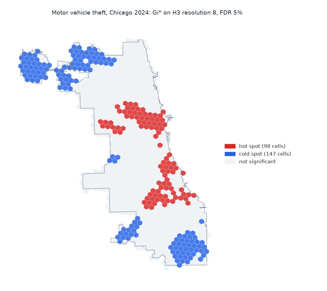
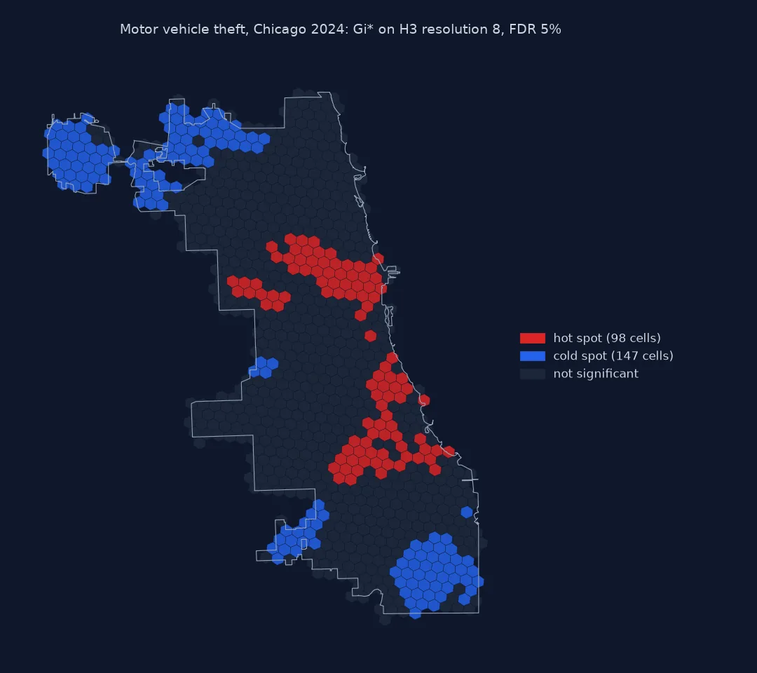
At an uncorrected 0.05, 152 of the 870 cells are hot spots and 210 cold spots. The cold spots outnumber the hot ones because most of the city has few thefts and the high counts are concentrated.

Map of Chicago on an H3 resolution 8 hexagon grid showing Gi* results for 2024 motor vehicle thefts after a 5 percent false discovery rate correction: 98 hot spot cells in red in two large clusters, one on the West and Near North Sides and one on the South Side, and 147 cold spot cells in blue at O'Hare, on the far north-west side, and in the far south-west and south-east of the city. — Hot and cold spots of motor vehicle theft.

A covering grid, corrected p-values, a checked resolution

1. Build a grid that covers the study area

Gi* compares each neighbourhood with the mean of all cells, so cells with no thefts are part of the data. Fill the city with cells, then add any cell that holds an incident but whose centre falls outside the boundary, so no incident is lost:

print(f"cells: {len(CELLS)}; with no thefts: {(CNT == 0).sum()}; most in one cell: {int(CNT.max())}")
print(f"thefts counted: {int(CNT.sum()):,} of {len(MVT):,}")
print(f"cells with no neighbour: {len(w.islands)}; connected parts: {w.n_components}")
areas = np.array([h3.cell_area(c, "km^2") for c in CELLS])
print(f"cell areas {areas.min():.4f} to {areas.max():.4f} km², a spread of {areas.max() / areas.min() - 1:.2%}")

cells: 870; with no thefts: 85; most in one cell: 129
thefts counted: 21,638 of 21,638
cells with no neighbour: 0; connected parts: 1
cell areas 0.7404 to 0.7453 km², a spread of 0.67%

Adding the cells that hold a theft but whose centres are outside the boundary brings every one of the 21,638 thefts into the grid. 85 cells, about one in ten, have none; they stay in.

2. Correct the p-values for multiple testing

With 999 permutations, each cell has its own pseudo p-value. Testing hundreds of cells at 0.05 flags some by chance; the false discovery rate procedure lowers the threshold so that, on average, no more than 5% of flagged cells are false:

thr = fdr(g.p_sim, 0.05)
hot_fdr = (g.Zs > 0) & (g.p_sim <= thr)
cold_fdr = (g.Zs < 0) & (g.p_sim <= thr)
print(f"FDR threshold: p <= {thr:.4f}")
print(f"hot spots {hot.sum()} -> {hot_fdr.sum()}, holding {CNT[hot_fdr].sum() / CNT.sum():.1%} of thefts; cold spots {cold.sum()} -> {cold_fdr.sum()}")

FDR threshold: p <= 0.0141
hot spots 152 -> 98, holding 27.2% of thefts; cold spots 210 -> 147

The correction removes about a third of the hot spots, 152 to 98, and the 98 that remain hold 27.2% of thefts in 11.3% of the city's cells.

Three maps of the same Gi* analysis at H3 resolutions 7, 8 and 9: 20, 98 and 542 hot cells; the hot spots sit in the same West Side and South Side areas at every resolution, breaking into finer, more fragmented patches at resolution 9, while cold spots stay on the north-west and far south edges. — The grid size changes the detail, not the pattern.

3. Check the resolution

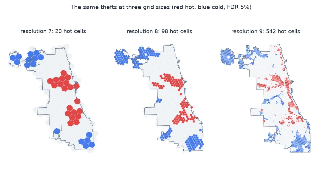
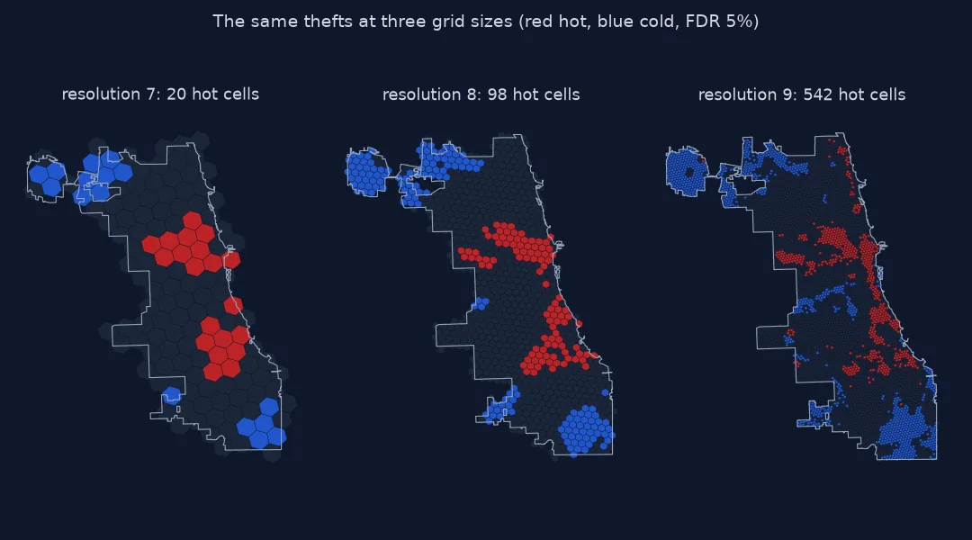
The grid is a choice. Run the same analysis at resolutions 7, 8 and 9, cells of about 5, 0.74 and 0.11 km²:

rows = []
for res in (7, 8, 9):
    cnt, cells = hex_counts(res)
    gr = G_Local(cnt.values.astype(float), h3_weights(cells), star=True, transform="B", permutations=999, seed=1)
    t = fdr(gr.p_sim, 0.05)
    hr = (gr.Zs > 0) & (gr.p_sim <= t)
    rows.append({"resolution": res, "cells": len(cells), "empty": int((cnt == 0).sum()), "hot (FDR)": int(hr.sum()),
                 "area share": f"{hr.mean():.1%}", "theft share": f"{cnt[hr].sum() / cnt.sum():.1%}"})
print(pd.DataFrame(rows).to_string(index=False))

 resolution  cells  empty  hot (FDR) area share theft share
          7    144      2         20      13.9%       28.3%
          8    870     85         98      11.3%       27.2%
          9   5694   1609        542       9.5%       27.0%

The number of hot cells changes with the grid, but the share of thefts they capture barely moves: 28.3%, 27.2% and 27.0%, from fewer, larger cells to more, smaller ones. Finer grids concentrate the same thefts into less area, 13.9% down to 9.5%.

Leaving out the empty cells

The data used on this page

The City of Chicago's Crimes - 2001 to Present dataset (ijzp-q8t2), motor vehicle thefts dated 2024 with coordinates, and the community area boundaries, dissolved into the city outline. Grid cells are H3 hexagons.

from pathlib import Path

import geopandas as gpd
import h3
import numpy as np
import pandas as pd
import requests
from esda import fdr
from esda.getisord import G_Local
from libpysal.weights import W

Path("data").mkdir(exist_ok=True)
URL = "https://data.cityofchicago.org/resource/ijzp-q8t2.json"
F = Path("data/chicago_crimes_2024.parquet")
if not F.exists():
    rows, offset = [], 0
    while True:
        part = requests.get(URL, timeout=300, params={
            "$where": "year=2024", "$limit": 50_000, "$offset": offset, "$order": "id",
            "$select": "id,date,primary_type,arrest,domestic,community_area,latitude,longitude,location_description,block,updated_on"}).json()
        rows += part; offset += len(part)
        if len(part) < 50_000:
            break
    pd.DataFrame(rows).to_parquet(F)
G = Path("data/chicago_community_areas.geojson")
if not G.exists():
    G.write_bytes(requests.get("https://data.cityofchicago.org/resource/igwz-8jzy.geojson?$limit=100", timeout=120).content)
MVT = pd.read_parquet(F).query("primary_type == 'MOTOR VEHICLE THEFT'").dropna(subset=["latitude", "longitude"])
MVT = MVT.astype({"latitude": float, "longitude": float})
CITY = gpd.read_file(G).union_all()


def hex_counts(res):
    """Thefts per H3 cell, over every cell in the city plus any cell holding a theft."""
    ids = [h3.latlng_to_cell(la, lo, res) for la, lo in zip(MVT.latitude, MVT.longitude)]
    cells = sorted(set(h3.geo_to_cells(h3.geo_to_h3shape(CITY.__geo_interface__), res)) | set(ids))
    return pd.Series(ids).value_counts().reindex(cells, fill_value=0), cells


def h3_weights(cells):
    """Binary weights: each cell's neighbours are the ring of six around it."""
    s = set(cells)
    return W({c: [n for n in h3.grid_disk(c, 1) if n != c and n in s] for c in cells}, silence_warnings=True)


print(f"{len(MVT):,} motor vehicle thefts with coordinates")

21,638 motor vehicle thefts with coordinates

Example 1: leave out the empty cells

A common shortcut is to aggregate the points and keep only the cells that have some. Run the same test on those cells alone:

nz = CNT[CNT > 0]
g_nz = G_Local(nz.values.astype(float), h3_weights(list(nz.index)), star=True, transform="B", permutations=999, seed=1)
t_nz = fdr(g_nz.p_sim, 0.05)
hot_nz = pd.Series((g_nz.Zs > 0) & (g_nz.p_sim <= t_nz), index=nz.index)
cold_nz = pd.Series((g_nz.Zs < 0) & (g_nz.p_sim <= t_nz), index=nz.index)
full_hot = pd.Series(hot_fdr, index=CNT.index)
print(f"mean per cell: {CNT.mean():.1f} with empty cells, {nz.mean():.1f} without")
print(f"hot spots: {full_hot.sum()} with empty cells, {hot_nz.sum()} without; in both: {(full_hot[nz.index] & hot_nz).sum()}")
print(f"cold spots: {cold_fdr.sum()} with empty cells, {cold_nz.sum()} without")

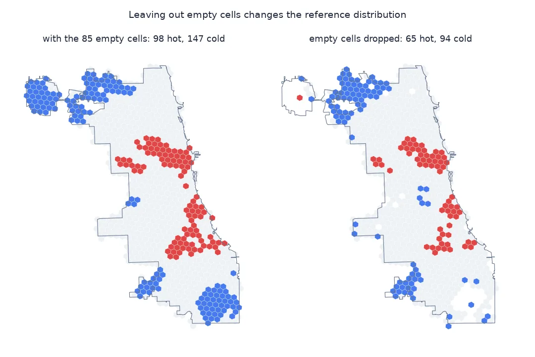
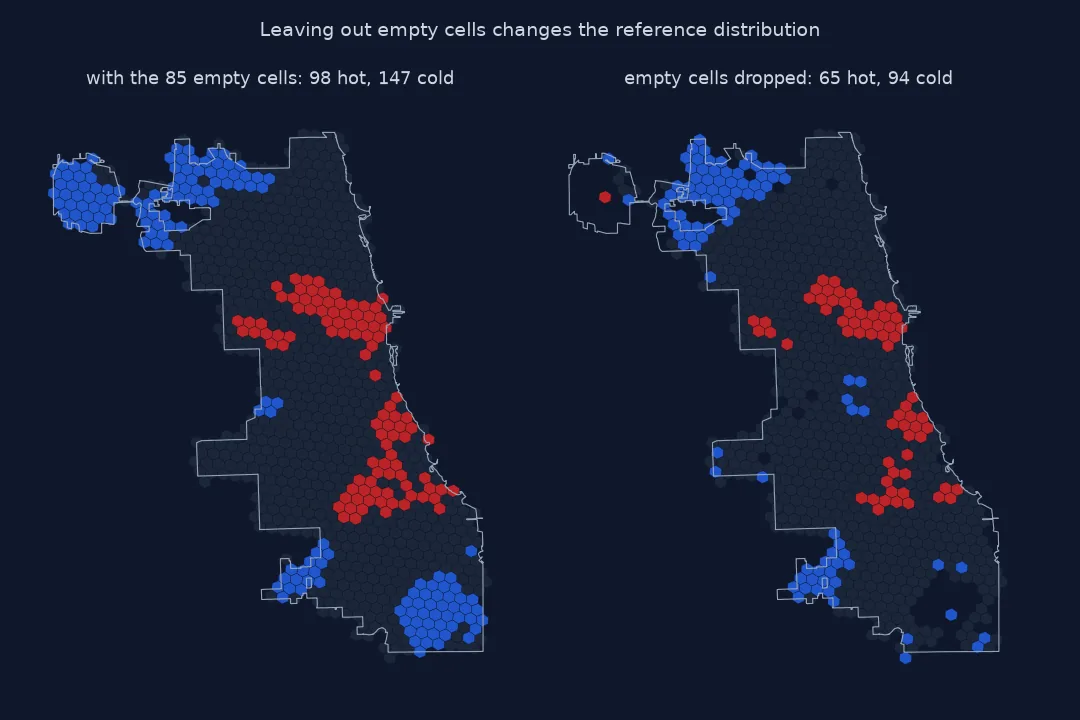
mean per cell: 24.9 with empty cells, 27.6 without
hot spots: 98 with empty cells, 65 without; in both: 64
cold spots: 147 with empty cells, 94 without

Dropping the 85 empty cells raises the mean from 24.9 to 27.6 thefts per cell and changes the answer: 65 hot spots instead of 98, and 94 cold spots instead of 147. Almost every hot spot found without the empty cells is also found with them, 64 of 65, the exception a cell at O'Hare; the shortcut mostly loses hot spots rather than inventing them.

Two maps of Gi* hot and cold spots for 2024 motor vehicle thefts at resolution 8: with the 85 empty cells, 98 hot and 147 cold; with them dropped, 65 hot and 94 cold, the hot clusters shrinking, the O'Hare and far south-east cold spots largely disappearing, and one cell at O'Hare turning hot. — Dropping empty cells changes the answer.

Gi* is a local statistic

From cells to corrected hot spots.

Gi* is a local statistic: for each cell, it adds up the values in the cell and its neighbours, and compares that sum with what it would be if the values were spread at random over the grid. A large positive z-score means the cell sits in a cluster of high counts; a large negative one, in a cluster of low counts. With star=True the cell itself is included in its own neighbourhood, which is the usual choice for hot spot mapping. The permutation p-value comes from reshuffling the counts over the cells many times and seeing how often a sum as extreme turns up.

The statistic is defined relative to the whole grid, which is why the grid matters. Leaving out empty cells raises the mean and removes the low-value neighbours that define cold spots; making cells larger smooths neighbourhoods together; and any grid has edges, where cells have fewer neighbours. None of these are errors in the method. They are parts of the question, and the result should be reported with them: the resolution, the treatment of empty cells, the number of permutations and the correction for multiple testing.

Gi* also says nothing about rates. A hot spot of motor vehicle theft is a cluster of high counts, which in a city often follows where cars are parked in large numbers. As with any crime map, the count is of recorded incidents.

Unequal H3 cells, islands and seeds

Gi* hotspot traps.

H3 cells are not equal-area: across a city the variation is well under a percent; across a continent it matters.
Islands: a cell with no neighbours, such as one isolated on the city's edge, gets no meaningful Gi*; check w.islands.
Disconnected parts: O'Hare is joined to the rest of Chicago by a narrow strip; check w.n_components, which is 1 here at resolution 8.
Seeds: permutation p-values vary slightly between runs; fix seed so results reproduce.
Distance bands instead of rings: libpysal.weights.DistanceBand gives the same test with a radius in metres on a projected grid.

Internal links

How to find hotspots with Getis-Ord Gi* in Python — Gi* in general
How to map crime hotspots with kernel density in Python — the density view
How to download and map city crime data in Python — the incidents

FAQ

How do I find crime hotspots with Gi* in Python?

Count incidents per grid cell, including empty cells, build spatial weights from cell adjacency, and run esda.getisord.G_Local(values, w, star=True, permutations=999); cells with positive Zs and small p_sim are hot spots.

Should I include cells with zero crimes?

Yes; they are part of the distribution Gi* compares against, and leaving them out raises the mean and hides cold spots.

Do I need to correct Gi* p-values?

When testing hundreds of cells, yes; esda.fdr(p_sim, 0.05) gives a false-discovery-rate threshold.

What grid size should I use for a hotspot analysis?

Try more than one: the hot spots should be broadly stable across resolutions, and the choice reported.