How to Compare Arrest Rates Between Areas in Python

Problem statement

The share of recorded incidents that end in an arrest varies a great deal from one neighbourhood to another, and a map of it is easy to read as a map of policing intensity or effectiveness. Most of the variation, though, comes from what is recorded where. Some offences, such as narcotics and weapons violations, are recorded almost only when police make an arrest; others, such as vehicle theft, almost never lead to one. An area with many of the first kind will have a high arrest share whatever its police do.

This page computes the arrest share of Chicago's 2024 recorded incidents by community area, adjusts it for each area's mix of offence types with indirect standardisation, the same method epidemiologists use for death rates, and finds which offence types drive the areas that remain high after adjustment.

Quick answer

Compute each type's city-wide arrest share, sum those shares over an area's incidents to get its expected arrests, and divide observed by expected:

CITY_SHARE = J.groupby("primary_type").arrest.mean()
J["expected"] = J.primary_type.map(CITY_SHARE)
A = J.groupby("community").agg(incidents=("arrest", "size"), arrests=("arrest", "sum"), expected=("expected", "sum"))
A["raw_share"] = A.arrests / A.incidents
A["ratio"] = A.arrests / A.expected                                  # 1 = what the city's type shares predict
print(f"city: {J.arrest.mean():.1%} of {len(J):,} incidents ended in an arrest")
print(A.sort_values("raw_share", ascending=False).head(4).round(3).to_string())

city: 13.8% of 256,654 incidents ended in an arrest
                    incidents  arrests  expected  raw_share  ratio
community                                                         
HUMBOLDT PARK            7035     1941  1841.962      0.276  1.054
WEST GARFIELD PARK       3699     1014   997.983      0.274  1.016
PULLMAN                  1042      245   143.080      0.235  1.712
NORTH LAWNDALE           6485     1392  1331.668      0.215  1.045

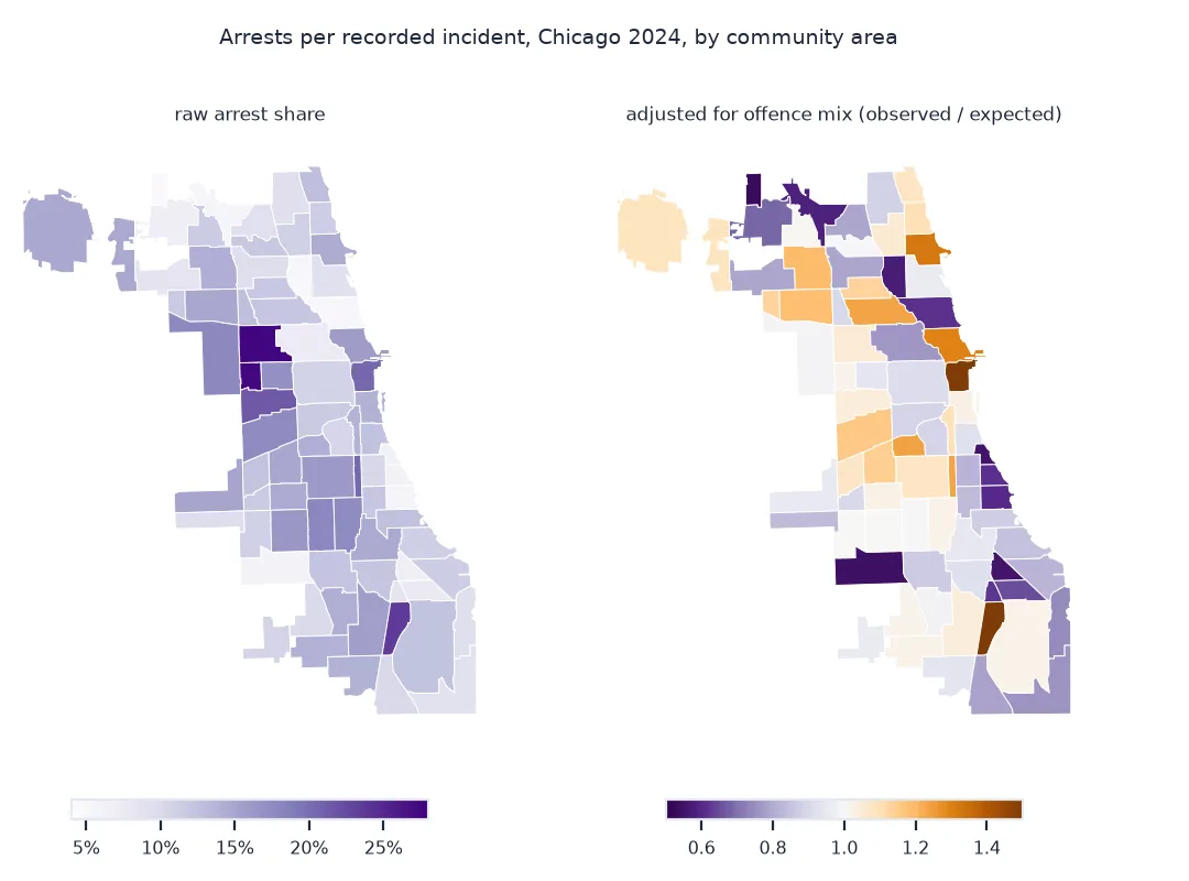
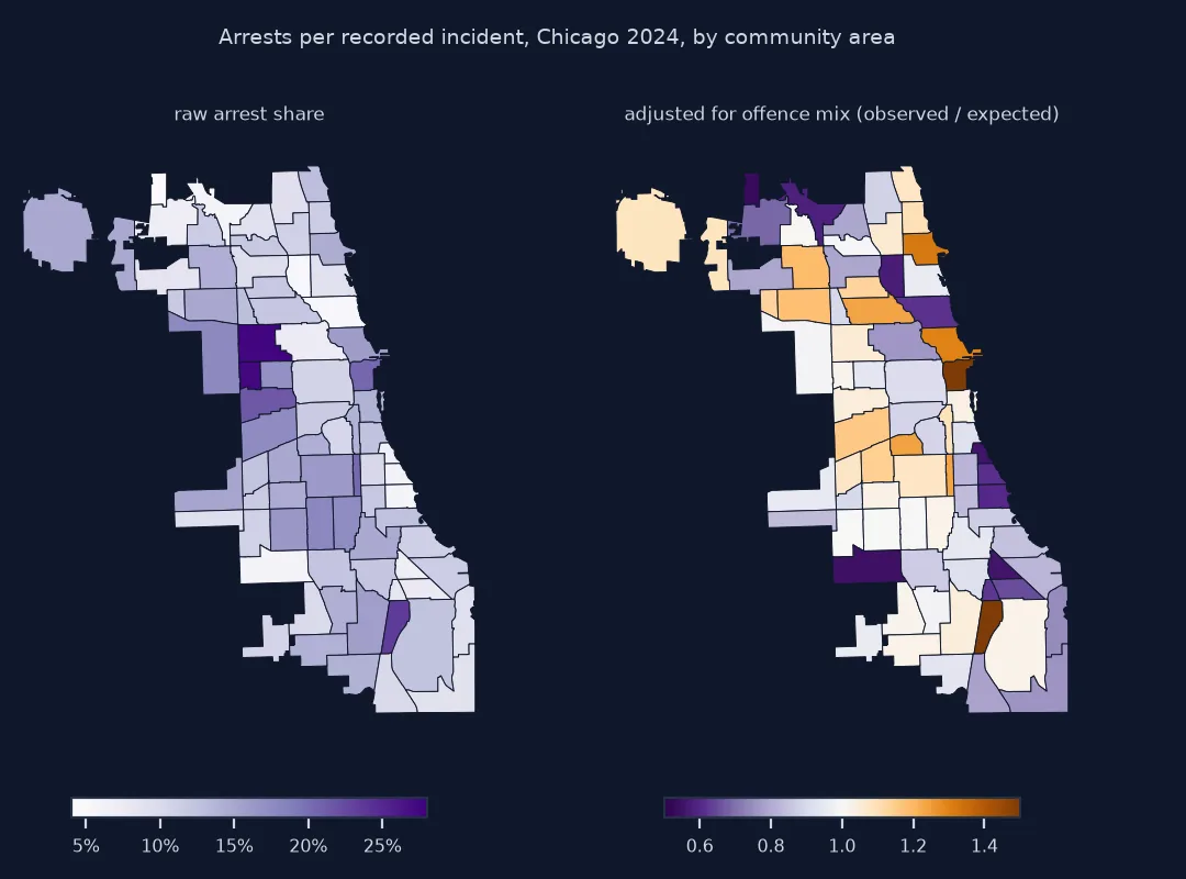
By raw share, Humboldt Park and West Garfield Park lead at about 27.5%, twice the city's 13.8%. Their adjusted ratios are 1.05 and 1.02: almost exactly what their mix of offence types predicts.

How much type mix explains, raw against adjusted, an interval

1. See how much the type mix explains

The narcotics share of an area's incidents alone tracks its arrest share closely:

A["narcotics_share"] = (J[J.primary_type == "NARCOTICS"].groupby("community").size() / A.incidents).reindex(A.index).fillna(0)
print(f"correlation of narcotics share with raw arrest share: {A.narcotics_share.corr(A.raw_share):.2f}")
print(A.loc[["WEST GARFIELD PARK", "HUMBOLDT PARK", "LINCOLN PARK"], ["raw_share", "narcotics_share"]].round(3).to_string())

correlation of narcotics share with raw arrest share: 0.75
                    raw_share  narcotics_share
community                                     
WEST GARFIELD PARK      0.274            0.138
HUMBOLDT PARK           0.276            0.154
LINCOLN PARK            0.052            0.002

Narcotics make up 13.8% and 15.4% of recorded incidents in West Garfield Park and Humboldt Park, against 0.2% in Lincoln Park, and the narcotics share alone correlates with the arrest share at 0.75.

2. Compare the raw and adjusted rankings

print(f"rank correlation of raw share and adjusted ratio: {A.raw_share.corr(A.ratio, method='spearman'):.2f}")
print(f"raw share: {A.raw_share.min():.1%} to {A.raw_share.max():.1%}; ratio: {A.ratio.min():.2f} to {A.ratio.max():.2f}")
print(A.sort_values("ratio", ascending=False).head(3)[["incidents", "arrests", "expected", "raw_share", "ratio"]].round(3).to_string())
print(A.sort_values("ratio").head(3)[["incidents", "arrests", "expected", "raw_share", "ratio"]].round(3).to_string())

rank correlation of raw share and adjusted ratio: 0.78
raw share: 4.6% to 27.6%; ratio: 0.53 to 1.71
           incidents  arrests  expected  raw_share  ratio
community                                                
PULLMAN         1042      245   143.080      0.235  1.712
LOOP            9286     1908  1245.996      0.205  1.531
UPTOWN          4546      657   496.334      0.145  1.324
             incidents  arrests  expected  raw_share  ratio
community                                                  
EDISON PARK        260       12    22.634      0.046  0.530
ASHBURN           2375      140   256.733      0.059  0.545
OAKLAND            860       55    99.803      0.064  0.551

Adjustment shrinks the range from sixfold, 4.6% to 27.6%, to about threefold, 0.53 to 1.71, and reorders the top: Pullman, the Loop and Uptown lead after adjustment, none of them in the raw top two.

3. Add an interval to the ratio

An observed-to-expected ratio is a count over a count. A Poisson interval on the observed arrests shows which ratios are clearly different from one:

from scipy.stats import chi2
A["lo"] = chi2.ppf(0.025, 2 * A.arrests) / 2 / A.expected
A["hi"] = chi2.ppf(0.975, 2 * (A.arrests + 1)) / 2 / A.expected
above, below = (A.lo > 1).sum(), (A.hi < 1).sum()
print(f"ratio clearly above 1: {above} areas; clearly below: {below}; interval includes 1: {len(A) - above - below}")
print(A.loc[["EDISON PARK", "LOOP"], ["arrests", "ratio", "lo", "hi"]].round(2).to_string())

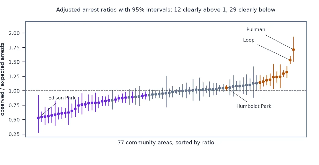
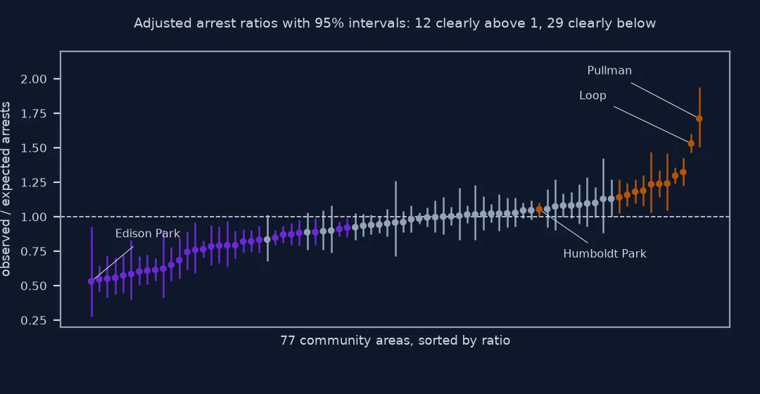
ratio clearly above 1: 12 areas; clearly below: 29; interval includes 1: 36
             arrests  ratio    lo    hi
community                              
EDISON PARK       12   0.53  0.27  0.93
LOOP            1908   1.53  1.46  1.60

Twelve areas are clearly above what their mix predicts and 29 clearly below; for 36 the interval includes one. Edison Park's ratio of 0.53 rests on 12 arrests, and its interval runs from 0.27 to 0.93; the Loop's 1.53 rests on 1,908 and is tightly estimated.

What drives a high arrest ratio

The data used on this page

The City of Chicago's Crimes - 2001 to Present dataset (ijzp-q8t2), incidents dated 2024 with coordinates and their arrest flag, which records whether an arrest was made, and the community area boundaries.

from pathlib import Path

import geopandas as gpd
import pandas as pd
import requests

Path("data").mkdir(exist_ok=True)
URL = "https://data.cityofchicago.org/resource/ijzp-q8t2.json"
F = Path("data/chicago_crimes_2024.parquet")
if not F.exists():
    rows, offset = [], 0
    while True:
        part = requests.get(URL, timeout=300, params={
            "$where": "year=2024", "$limit": 50_000, "$offset": offset, "$order": "id",
            "$select": "id,date,primary_type,arrest,domestic,community_area,latitude,longitude,location_description,block,updated_on"}).json()
        rows += part; offset += len(part)
        if len(part) < 50_000:
            break
    pd.DataFrame(rows).to_parquet(F)
G = Path("data/chicago_community_areas.geojson")
if not G.exists():
    G.write_bytes(requests.get("https://data.cityofchicago.org/resource/igwz-8jzy.geojson?$limit=100", timeout=120).content)
c = pd.read_parquet(F).dropna(subset=["latitude", "longitude"]).assign(arrest=lambda d: d.arrest.astype(bool))
pts = gpd.GeoDataFrame(c, geometry=gpd.points_from_xy(c.longitude.astype(float), c.latitude.astype(float)), crs=4326)
CA = gpd.read_file(G)
J = gpd.sjoin(pts, CA[["community", "geometry"]], predicate="within")
print(f"{len(J):,} incidents in {J.community.nunique()} community areas; {J.primary_type.nunique()} offence types")

256,654 incidents in 77 community areas; 31 offence types

Example 1: what drives a high ratio

For the areas with the highest adjusted ratios, the excess arrests by offence type, observed minus expected:

for area in A.sort_values("ratio", ascending=False).index[:2]:
    a = J[J.community == area]
    by = a.groupby("primary_type").agg(n=("arrest", "size"), arrests=("arrest", "sum"), expected=("expected", "sum"))
    by["excess"] = by.arrests - by.expected
    print(f"{area.title()}: {A.loc[area, 'arrests']:.0f} arrests, {A.loc[area, 'expected']:.0f} expected")
    print(by.sort_values("excess", ascending=False).head(3).round(1).to_string())

Pullman: 245 arrests, 143 expected
                     n  arrests  expected  excess
primary_type                                     
THEFT              275      118      18.4    99.6
ASSAULT            130       20      14.0     6.0
CRIMINAL TRESPASS   16        7       4.6     2.4
Loop: 1908 arrests, 1246 expected
                       n  arrests  expected  excess
primary_type                                       
THEFT               3669      571     245.9   325.1
DECEPTIVE PRACTICE  1014      137      34.4   102.6
BATTERY             1182      268     202.7    65.3

Almost all of Pullman's excess is theft: 118 arrests on 275 thefts against 18 expected. In the Loop, theft and deceptive practice together account for 428 of the 662 extra arrests. Theft covers shoplifting and other kinds; the description field would show which kind these are.

Indirect standardisation of arrests

Indirect standardisation asks: if every offence type in this area ended in arrest as often as it does across the city, how many arrests would there be? The answer, the expected count, carries the area's type mix and nothing else. Dividing the observed arrests by it leaves what the mix does not explain. A ratio above one means more arrests than the city's type-by-type shares predict, below one fewer. The same arithmetic produces standardised mortality ratios, with age groups in place of offence types.

The adjustment shrinks the range a great deal and reorders the map. Areas on the West Side with high raw arrest shares turn out to be close to what their incident mix predicts, because a large share of their recorded incidents are narcotics and weapons offences, recorded mostly through arrests. What remains after adjustment is a smaller set of real differences, which still need explaining case by case; an excess concentrated in one offence type, as Pullman's is in theft, points to how that offence is detected there rather than to policing in general.

Neither the raw nor the adjusted figure measures how well crimes are solved. The arrest flag records whether an arrest was made, not whether the arrested person committed the offence; many offences are never reported at all; and offences discovered through police activity are, by construction, recorded together with an arrest.

Finer types, late arrests and small areas

• Finer types: standardising on primary_type leaves variation within types, such as retail theft against other theft; the description field allows a finer adjustment.
• Arrests made later: the flag can change as investigations proceed; a download soon after the year ends will show fewer arrests than one made months later.
• Arrests dataset: Chicago publishes a separate arrests dataset, one row per arrest, which is not linked to incidents one to one.
• Small areas: Edison Park's 260 incidents give a wide interval; show intervals, or pool years.
• Direct standardisation: applying each area's type shares to a standard mix is the alternative; it needs every type in every area, which rare types break.

Internal links

• How to download and map city crime data in Python — arrests by offence type
• How to calculate crime rates per resident in Python — rates and denominators
• How to calculate age-adjusted rates in Python — the same standardisation for health data

FAQ

How do I compare arrest rates between neighbourhoods?

Adjust for the mix of offence types: compute each type's city-wide arrest share, sum those shares over each area's incidents to get expected arrests, and compare observed with expected.

Why are arrest rates higher in some areas?

Mostly because of what is recorded there: offences such as narcotics are recorded almost only with an arrest, so areas where many are recorded have high arrest shares.

What is indirect standardisation?

A way of comparing a rate across groups with different compositions: apply reference rates for each category to each group's composition, and divide observed by expected.

Does a high arrest rate mean better policing?

No; it reflects the offence mix, reporting and police activity together, and says nothing on its own about whether crimes were solved correctly.