
How to Analyse Crime Trends Over Time in Python
On this page
Problem statement
"Is crime going up?" is the question every crime dataset is asked first, and the one most easily answered wrongly. A monthly series of recorded incidents mixes the trend with the season, ends in a month that is not yet complete, and adds together offence types moving in opposite directions. Across a city, the change in one neighbourhood can be the reverse of the change in the next.
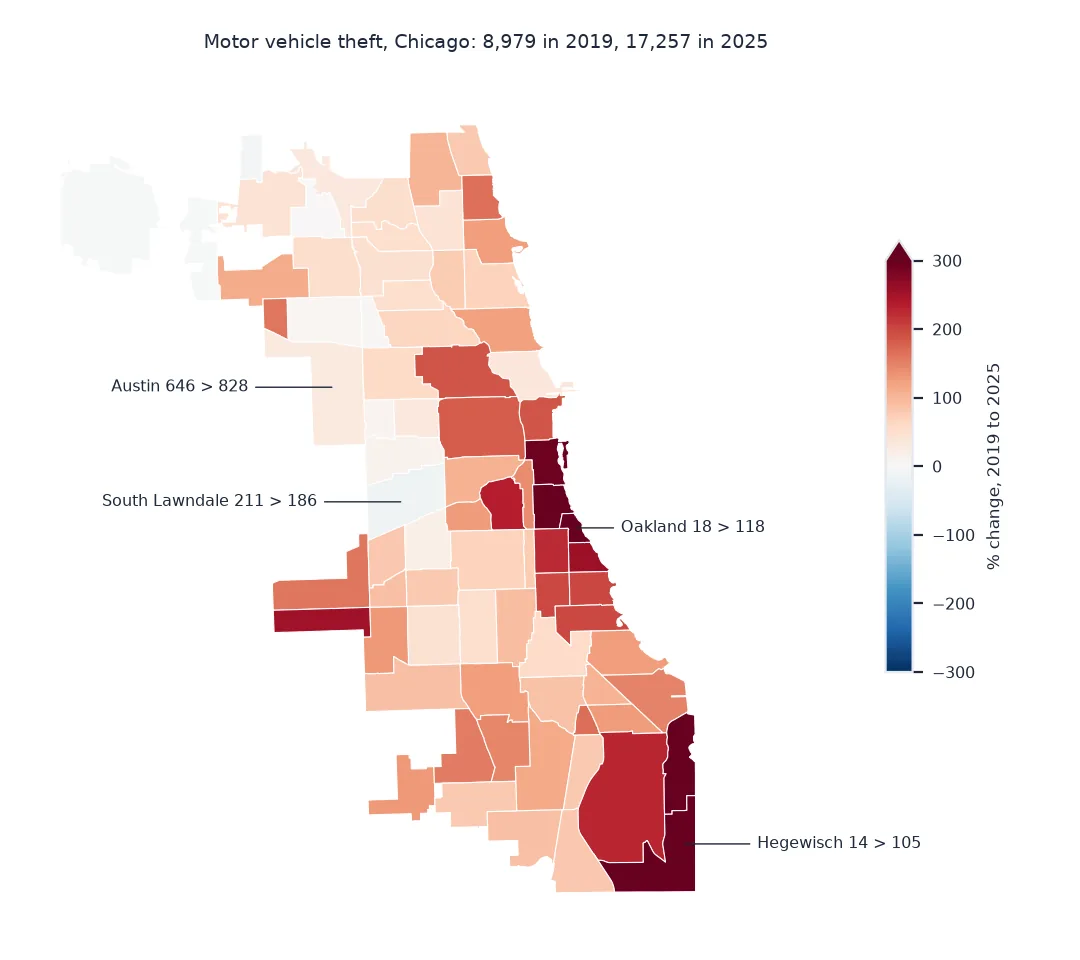
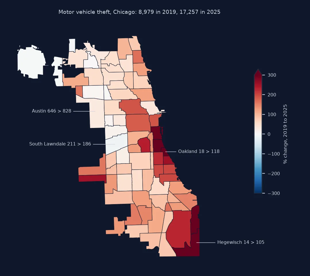
This page pulls monthly counts of every recorded incident in Chicago from January 2019 with Socrata's server-side aggregation, removes the incomplete months at the end, separates season from trend with a twelve-month rolling sum, compares offence types, and maps the change in motor vehicle theft by community area between 2019 and 2025.
Quick answer
Ask the API for counts rather than rows, drop months that are not complete, and compare whole years or rolling twelve-month totals:
M = MONTHLY[MONTHLY.month <= LAST_FULL].groupby("month").n.sum()
roll = M.rolling(12).sum()
print(f"{M.index.min():%b %Y} to {M.index.max():%b %Y}: {len(M)} complete months")
print(f"12 months to {M.index.max():%b %Y}: {roll.iloc[-1]:,.0f} incidents; a year earlier: {roll.iloc[-13]:,.0f} ({roll.iloc[-1] / roll.iloc[-13] - 1:+.1%})")
print(M.groupby(M.index.year).sum().loc[2019:2025].to_string())
Jan 2019 to Aug 2026: 92 complete months
12 months to Aug 2026: 232,609 incidents; a year earlier: 245,532 (-5.3%)
month
2019 261938
2020 213071
2021 210002
2022 240496
2023 263846
2024 259638
2025 238100
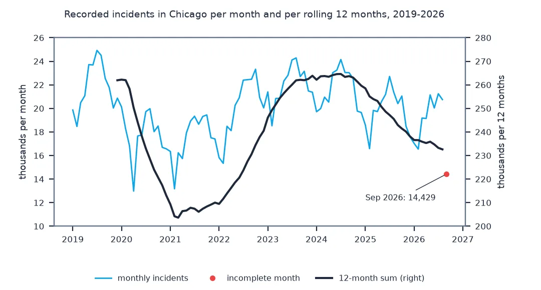
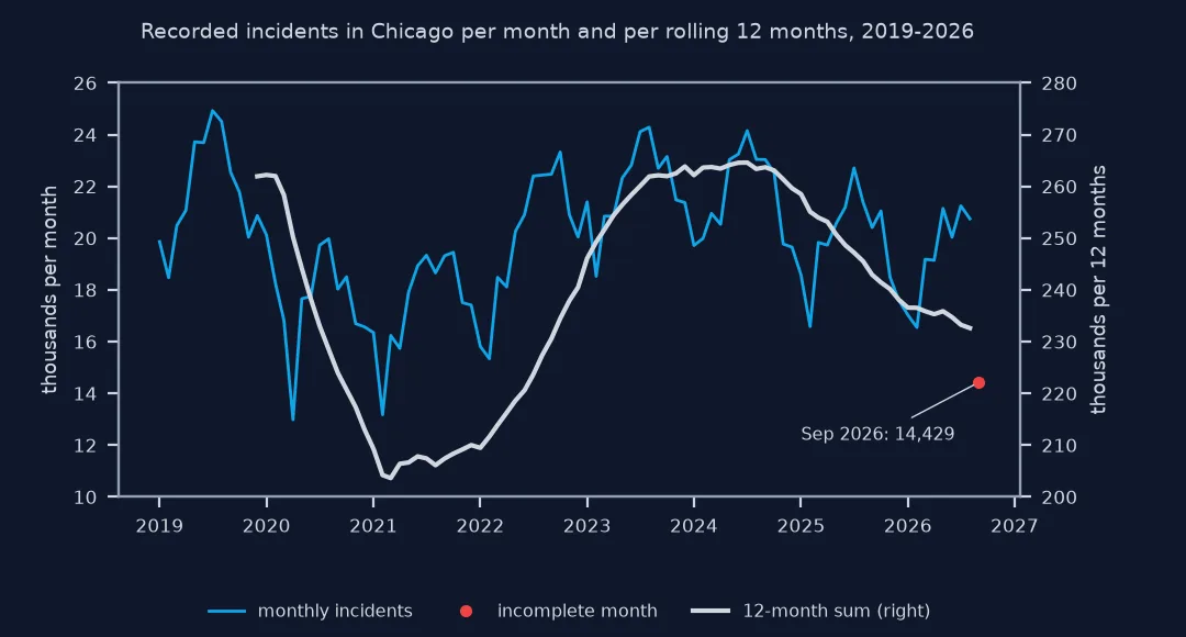
Recorded incidents fell by a fifth from 2019 to 2020 and 2021, returned to the 2019 level in 2023 and 2024, and fell again in 2025. The twelve months to August 2026 are 5.3% below the twelve months before.
The last complete month, season against trend, split by type
1. Find the last complete month
The dataset leaves out the most recent seven days, and the current month is partial anyway. Compare the last months with the same months a year earlier before trusting them:
tot = MONTHLY.groupby("month").n.sum()
for m in tot.index[-3:]:
    prev = tot.get(m - pd.DateOffset(years=1))
    print(f"{m:%b %Y}: {tot[m]:,} incidents; {m - pd.DateOffset(years=1):%b %Y}: {prev:,} ({tot[m] / prev - 1:+.0%})")
print(f"data updated {UPDATED:%d %b %Y}; last complete month used: {LAST_FULL:%b %Y}")
Jul 2026: 21,245 incidents; Jul 2025: 22,712 (-6%)
Aug 2026: 20,745 incidents; Aug 2025: 21,386 (-3%)
Sep 2026: 14,429 incidents; Sep 2025: 20,406 (-29%)
data updated 01 Oct 2026; last complete month used: Aug 2026
September 2026 looks like a 29% fall, and is an artefact: the data were updated on 1 October and the last seven days are withheld. July and August are complete and show falls of 6% and 3%.
2. Separate the season from the trend
Crime in Chicago has a strong season. Comparing a summer month with a winter month says nothing about the trend:
season = M.groupby(M.index.month).mean()
print(f"busiest calendar month on average: {pd.Timestamp(2000, season.idxmax(), 1):%B} ({season.max():,.0f}); "
      f"quietest: {pd.Timestamp(2000, season.idxmin(), 1):%B} ({season.min():,.0f}), {season.max() / season.min() - 1:.0%} apart")
print(f"largest month-to-month change: {M.pct_change().abs().max():.0%}; largest change in the 12-month sum: {roll.pct_change().abs().max():.1%}")
busiest calendar month on average: July (22,325); quietest: February (17,109), 30% apart
largest month-to-month change: 36%; largest change in the 12-month sum: 3.1%
July averages 30% more incidents than February. Month-to-month changes reach 36%; the twelve-month sum never moves by more than 3.1% in a month, because each step swaps one month for the same month a year earlier.
3. Split the total by offence type
Y = MONTHLY[MONTHLY.month.dt.year.between(2019, 2025)].pivot_table(index="primary_type", columns=MONTHLY.month.dt.year, values="n", aggfunc="sum")
types = ["THEFT", "BATTERY", "ASSAULT", "MOTOR VEHICLE THEFT", "ROBBERY", "BURGLARY", "NARCOTICS", "HOMICIDE"]
change = (Y[2025] / Y[2019] - 1).loc[types]
print(Y.loc[types, [2019, 2021, 2023, 2025]].astype(int).assign(change_2019_2025=change.map("{:+.0%}".format)).to_string())
month 2019 2021 2023 2025 change_2019_2025
primary_type
THEFT 62505 40830 57527 55198 -12%
BATTERY 49556 40512 44303 42660 -14%
ASSAULT 20626 20347 22643 21600 +5%
MOTOR VEHICLE THEFT 8979 10605 29256 17258 +92%
ROBBERY 7997 7923 11059 5815 -27%
BURGLARY 9638 6662 7494 9740 +1%
NARCOTICS 15080 5420 5455 7419 -51%
HOMICIDE 509 813 638 440 -14%
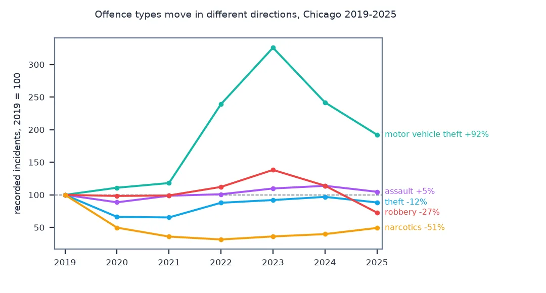
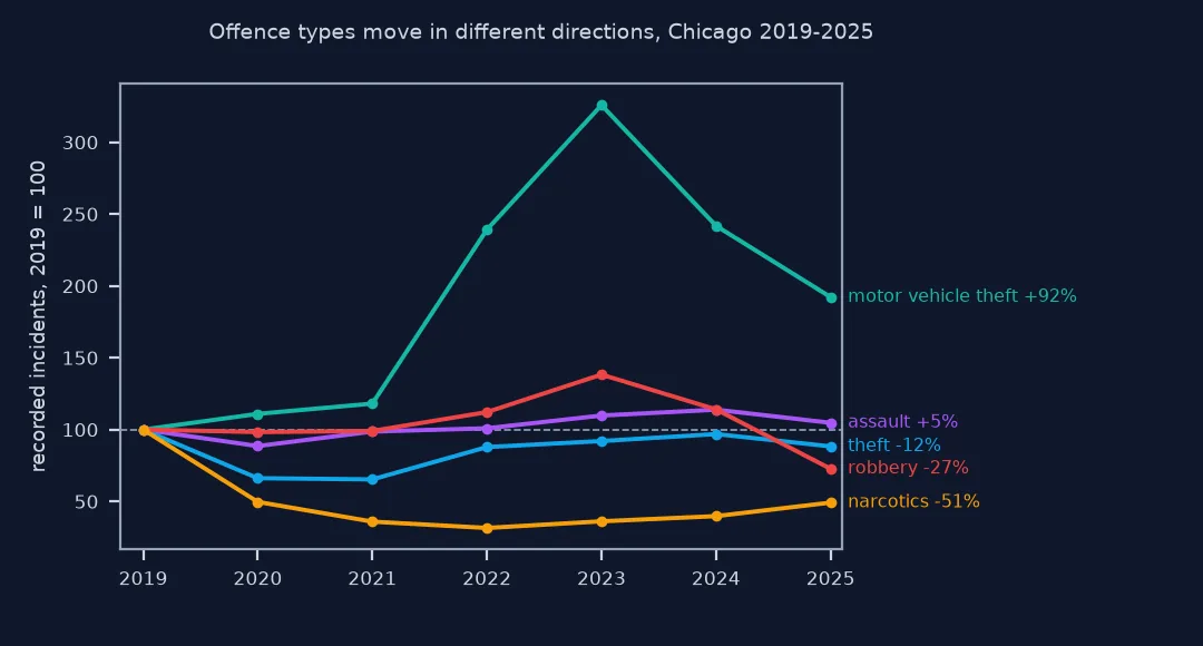
The total hides opposite movements. Motor vehicle theft rose 92% from 2019 to 2025, after more than tripling to 29,256 in 2023; narcotics fell by half and robbery by 27%. Narcotics incidents are recorded mostly when police find them, so their fall may reflect enforcement as much as offending.
Where motor vehicle theft changed
The data used on this page
The City of Chicago's Crimes - 2001 to Present dataset (ijzp-q8t2), aggregated on the server with SoQL $group: incidents per month and offence type from January 2019, and motor vehicle thefts per community area in 2019 and 2025; and the community area boundaries. Counts are as published on the download date.
from pathlib import Path

import geopandas as gpd
import pandas as pd
import requests

Path("data").mkdir(exist_ok=True)
URL = "https://data.cityofchicago.org/resource/ijzp-q8t2.json"


def soql(name, **params):
    f = Path(f"data/{name}.parquet")
    if not f.exists():
        pd.DataFrame(requests.get(URL, params={"$limit": 50_000, **params}, timeout=300).json()).to_parquet(f)
    return pd.read_parquet(f)


MONTHLY = soql("chicago_monthly_by_type", **{"$select": "date_trunc_ym(date) AS month, primary_type, count(*) AS n",
                                             "$where": "year >= 2019", "$group": "month, primary_type"})
MONTHLY = MONTHLY.astype({"n": int}).assign(month=lambda d: pd.to_datetime(d.month))
AREA = soql("chicago_mvt_by_area", **{"$select": "year, community_area, count(*) AS n",
                                      "$where": "primary_type = 'MOTOR VEHICLE THEFT' AND year IN (2019, 2025)",
                                      "$group": "year, community_area"}).astype({"n": int, "year": int})
f = Path("data/updated.txt")
if not f.exists():
    f.write_text(str(requests.get("https://data.cityofchicago.org/api/views/ijzp-q8t2.json", timeout=60).json()["rowsUpdatedAt"]))
UPDATED = pd.Timestamp(int(f.read_text()), unit="s")
LAST_FULL = (UPDATED - pd.Timedelta(days=7)).to_period("M").to_timestamp() - pd.DateOffset(months=1)
G = Path("data/chicago_community_areas.geojson")
if not G.exists():
    G.write_bytes(requests.get("https://data.cityofchicago.org/resource/igwz-8jzy.geojson?$limit=100", timeout=120).content)
CA = gpd.read_file(G).astype({"area_numbe": int})
print(f"{len(MONTHLY):,} month-type rows, {MONTHLY.n.sum():,} incidents; {len(AREA)} area-year rows")
2,659 month-type rows, 1,856,587 incidents; 155 area-year rows
Example 1: where motor vehicle theft changed
The city-wide change hides a range of local ones. Compare 2019 with 2025 by community area, keeping the counts beside the percentages:
A = AREA.dropna(subset=["community_area"]).astype({"community_area": int}).pivot(index="community_area", columns="year", values="n")
print(f"thefts with no valid area code (0 or missing): {AREA[~AREA.community_area.astype(float).isin(CA.area_numbe)].n.sum()}")
A = A.join(CA.set_index("area_numbe").community, how="inner").fillna({2019: 0, 2025: 0}).astype({2019: int, 2025: int})
A["change"] = A[2025] / A[2019] - 1
print(f"city: {A[2019].sum():,} in 2019, {A[2025].sum():,} in 2025 ({A[2025].sum() / A[2019].sum() - 1:+.0%})")
print(f"areas up: {(A.change > 0).sum()} of {len(A)}; more than doubled: {(A.change > 1).sum()}; down: {(A.change < 0).sum()}")
print(A.sort_values("change")[["community", 2019, 2025, "change"]].iloc[[0, 1, -2, -1]].round(2).to_string(index=False))
thefts with no valid area code (0 or missing): 1
city: 8,979 in 2019, 17,257 in 2025 (+92%)
areas up: 73 of 77; more than doubled: 37; down: 3
community 2019 2025 change
SOUTH LAWNDALE 211 186 -0.12
EDISON PARK 11 10 -0.09
OAKLAND 18 118 5.56
HEGEWISCH 14 105 6.50
Motor vehicle theft rose in 73 of 77 community areas and more than doubled in 37. The largest percentage rises are in areas with small 2019 bases: Hegewisch went from 14 to 105, Oakland from 18 to 118.
Offending, reporting and recording at once
A trend in recorded crime is a trend in three things at once: offending, reporting and recording. A rise in motor vehicle theft can be more cars stolen, more owners reporting thefts for insurance, or a change in how attempted thefts are classified. The data cannot separate these on its own, which is why a careful trend statement names the series exactly: recorded incidents of a type, as published on a date.
The mechanics are simpler. Use complete periods only. Compare like with like: the same months a year apart, whole years, or a rolling twelve-month total, which removes the season by always containing one of each month. Split totals into types before concluding anything, because a total is a sum of series that can move in opposite directions, and a large type dominates it. And when mapping change by area, show the counts as well as the percentages, because a small base turns a handful of incidents into a dramatic percentage.
Revised records, boundaries and month lengths
- Records change after publication: classifications and locations are revised, so last year's counts downloaded today differ slightly from the same counts downloaded last year.
- Boundary changes: community areas have been stable for decades; police districts and beats have not.
- Leap years and month lengths: February has fewer days; use rates per day when comparing single months.
- Events: one-off events, such as the 2020 pandemic lockdowns, are part of the series; a rolling sum spreads them over twelve months.
- The city's warning: the dataset description cautions against comparisons over time; it does not forbid them, but it is a reason to state the caveats.
Internal links
- How to download and map city crime data in Python — the dataset and its description
- How to calculate crime rates per resident in Python — rates instead of counts
- How to analyse crime by hour and day of week in Python — patterns within the day
FAQ
How do I get monthly crime counts from a Socrata API?
Use SoQL aggregation: $select=date_trunc_ym(date) AS month, count(*) AS n with $group=month, so the server returns counts instead of every row.
Why does the latest month always show a drop?
Because it is incomplete: Chicago withholds the most recent seven days, and the current month has not finished. Use complete months only.
How do I remove seasonality from a crime trend?
Compare the same months in different years, or use a rolling twelve-month sum, which always contains one of each month.
Did motor vehicle theft rise in Chicago?
Yes: recorded motor vehicle thefts rose from 8,979 in 2019 to 17,258 in 2025, after peaking at 29,256 in 2023.