
How to Measure Change from an Old Map in Python
On this page
Problem statement
The point of putting an old map on today's grid is usually to ask what has changed: how much woodland was lost, how far a coast retreated, which village disappeared. The overlay makes change easy to see and easy to overstate. Every number from it mixes real change with three kinds of error — the old survey's, the georeferencing's and the digitising's — and with the fact that "wood" on an 1880s sheet and "forest" in OpenStreetMap are not the same definition.
This page measures what happened to the woods of the Hambleton valley in Rutland between the Ordnance Survey six-inch survey of 1884–1891 and today, when much of the valley lies under Rutland Water, and reports each answer as a range that carries those errors.
Quick answer
Overlay the old polygons on today's data, split them by fate, and repeat the split under the uncertainty you know about — here, a 20 m georeferencing error and the digitising threshold:
def fate(old):
    o = old.union_all()
    water = o.intersection(WATER).area
    wood = o.difference(WATER).intersection(FOREST).area
    return {"old ha": o.area / 1e4, "under water": water / o.area, "still wood": wood / o.area,
            "now neither": 1 - (water + wood) / o.area}

runs = {f"threshold {t}, shift {s:+} m": fate(woods_1880s(t).buffer(s)) for t in (0.03, 0.04, 0.05) for s in (-20, 0, 20)}
table = pd.DataFrame(runs).T
print(table.loc["threshold 0.04, shift +0 m"].round(3).to_string())
print(table.agg(["min", "max"]).round(3).to_string())
old ha 124.738
under water 0.403
still wood 0.403
now neither 0.194
old ha under water still wood now neither
min 48.021 0.374 0.323 0.174
max 200.333 0.435 0.447 0.241
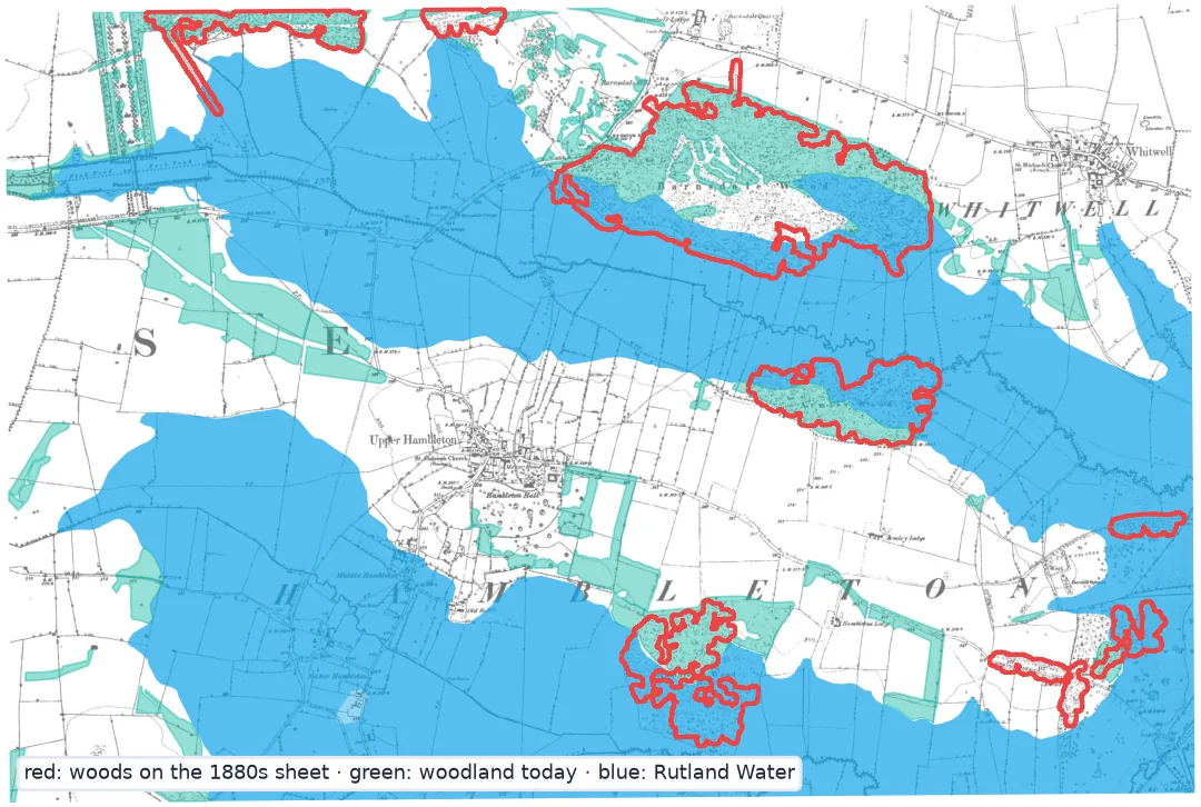
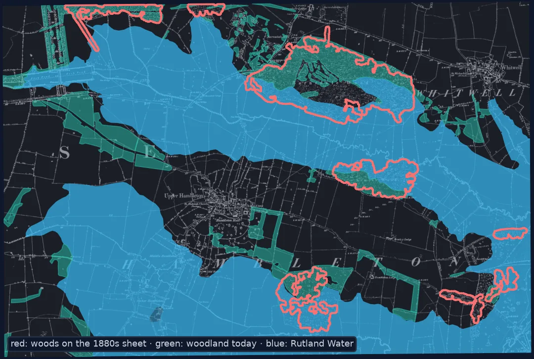
Of the woods on the 1880s sheet, roughly two-fifths are now under the reservoir, two-fifths are still woodland and one-fifth is neither — and those shares move by only about six percentage points either way whatever reasonable choices are made:
One grid, one definition, overlay, carry the errors
1. Put both dates on one grid
The 1880s woods were digitised from the tree stipple on sheet 009-NE, placed in British National Grid from sheet 009-NW's seven control points and the sheet layout (see digitising and mosaicking). Today's woodland and water come from OpenStreetMap, clipped to the same sheet:
print(f"sheet {SHEET.area / 1e4:,.0f} ha; Rutland Water on it {WATER.area / 1e4:,.0f} ha; "
      f"OSM woodland on it {FOREST.area / 1e4:,.0f} ha; 1880s woods {woods_1880s(0.04).area.sum() / 1e4:,.1f} ha")
sheet 1,552 ha; Rutland Water on it 700 ha; OSM woodland on it 144 ha; 1880s woods 124.7 ha
Almost half the sheet is now water. The reservoir was built in the 1970s by damming the Gwash valley, and the Hambleton peninsula is what remained above it.
2. Agree what "woodland" means at both dates
The old sheet draws woods as a stipple of tree symbols, bounded where the surveyor saw the wood end. OpenStreetMap's landuse=forest is drawn by volunteers from aerial imagery and includes plantations, shelterbelts and some parkland. Neither is a forestry inventory. The comparison is between two maps' ideas of woodland, and that should be said whenever the numbers are quoted.
3. Overlay and classify
Each piece of 1880s wood falls into one of three fates — under water, still woodland, neither — and the overlay gives the area of each, shown at the top of the page. It also gives the reverse: woodland today that was not woodland then:
o = woods_1880s(0.04).union_all()
new = FOREST.difference(o)
print(f"woodland today: {FOREST.area / 1e4:.1f} ha, of which {new.area / 1e4:.1f} ha was not wood in the 1880s "
      f"({new.area / FOREST.area:.0%})")
woodland today: 144.1 ha, of which 93.8 ha was not wood in the 1880s (65%)
Most of today's woodland on the sheet is new — plantations along the reservoir shore and around Upper Hambleton. The valley lost old woods to the water and gained new ones around it.
4. Carry the errors through
Two errors are known and can be simulated. The georeferencing is good to about 20 m (leave-one-out and three check churches); shrinking and growing every old polygon by 20 m brackets it. The digitising threshold moves woodland area by tens of hectares; repeating at 0.03 and 0.05 brackets that. The quick answer ran all nine combinations:
print(table[["old ha", "under water", "still wood"]].round(2).to_string()) old ha under water still wood
threshold 0.03, shift -20 m 105.52 0.41 0.40
threshold 0.03, shift +0 m 153.32 0.42 0.38
threshold 0.03, shift +20 m 200.33 0.44 0.32
threshold 0.04, shift -20 m 80.71 0.39 0.41
threshold 0.04, shift +0 m 124.74 0.40 0.40
threshold 0.04, shift +20 m 165.79 0.41 0.36
threshold 0.05, shift -20 m 48.02 0.37 0.44
threshold 0.05, shift +0 m 89.95 0.38 0.45
threshold 0.05, shift +20 m 126.00 0.39 0.42
The areas swing widely — the total old woodland ranges from 48 to 200 ha across the nine runs, a factor of four — but the shares barely move. That is the useful finding: the proportions are robust, the hectares are not.
5. Report the range, and the definitions
The defensible statement is a range of shares with its sources: "of the woods drawn on the 1884–1891 six-inch sheet 009-NE, 37–44% by area now lie under Rutland Water and 32–45% are still woodland in OpenStreetMap (1 January 2026)", with the range taken from the table. A single area to the hectare would claim a precision the map does not have.
Woodland change, wood by wood
The data used on this page
Ordnance Survey six-inch sheets Rutland 009-NW and 009-NE (1884–1891) from Wikimedia Commons (public domain); OpenStreetMap from Geofabrik (1 January 2026; © OpenStreetMap contributors, ODbL): landuse=forest and water areas over 100 ha.
from pathlib import Path

import geopandas as gpd
import numpy as np
import pandas as pd
import requests
from PIL import Image
from rasterio import features
from scipy import ndimage as ndi
from shapely import affinity
from shapely.geometry import Polygon, shape

Path("data").mkdir(exist_ok=True)
UA = {"User-Agent": "spatialworkflow.io guide (https://www.spatialworkflow.io)"}
COMMONS = "https://upload.wikimedia.org/wikipedia/commons/"
for name, path in {"009-NW": "a/a0/", "009-NE": "8/80/"}.items():
    if not Path(f"data/os_{name}.jpg").exists():
        url = f"{COMMONS}{path}Map_of_Rutland_OS_Map_name_{name}%2C_Ordnance_Survey%2C_1884-1891.jpg"
        Path(f"data/os_{name}.jpg").write_bytes(requests.get(url, headers=UA, timeout=300).content)
if not Path("data/rutland.shp.zip").exists():
    Path("data/rutland.shp.zip").write_bytes(requests.get(
        "https://download.geofabrik.de/europe/united-kingdom/england/rutland-260101-free.shp.zip",
        headers=UA, timeout=300).content)

GCPS = [  # (id, pixel, line, easting, northing) on 009-NW
    ("oakham_church",          3141,  487, 486065.6, 308906.1),
    ("egleton_church",         4824, 2031, 487598.5, 307540.3),
    ("brooke_rd_crossing",     2956, 1159, 485892.0, 308306.8),
    ("egleton_level_crossing", 3998, 2481, 486838.1, 307119.0),
    ("stamford_rd_guide_post", 5127,  988, 487872.3, 308486.1),
    ("braunston_rd_bridleway", 1263, 1675, 484382.4, 307839.2),
    ("brooke_guide_post",      1547, 3292, 484648.2, 306376.1),
]
X = np.array([[1, g[1], g[2]] for g in GCPS], float)
A = np.linalg.lstsq(X, np.array([[g[3], g[4]] for g in GCPS]), rcond=None)[0]
(w0, h0), (w, h) = Image.open("data/os_009-NW.jpg").size, Image.open("data/os_009-NE.jpg").size
sx, sy = w0 / w, h0 / h                                  # 009-NE is the next sheet east
NE = [A[1, 0] * sx, A[2, 0] * sy, A[1, 1] * sx, A[2, 1] * sy, A[0, 0] + A[1, 0] * w0, A[0, 1] + A[1, 1] * w0]
SHEET = affinity.affine_transform(Polygon([(0, 0), (w, 0), (w, h), (0, h)]), NE)

im = np.asarray(Image.open("data/os_009-NE.jpg").convert("L"))
lab, _ = ndi.label(im < 128)
sizes = np.bincount(lab.ravel())
is_dot = (sizes >= 2) & (sizes <= 40)
is_dot[0] = False
DENSITY = ndi.uniform_filter(is_dot[lab].astype(float), size=41)
yy, xx = np.ogrid[-15:16, -15:16]

def woods_1880s(threshold):
    """Woodland on sheet 009-NE from the tree stipple, as in the digitising guide."""
    m = ndi.binary_fill_holes(ndi.binary_opening(DENSITY > threshold, structure=xx**2 + yy**2 <= 225))
    L, k = ndi.label(m)
    m = np.r_[False, ndi.maximum(ndi.distance_transform_edt(m), L, range(1, k + 1)) >= 35][L]
    g = gpd.GeoSeries([affinity.affine_transform(shape(p), NE) for p, _ in features.shapes(m.astype(np.uint8), mask=m)],
                      crs=27700)
    return g[g.area > 2e4]

bb = tuple(gpd.GeoSeries([SHEET], crs=27700).to_crs(4326).total_bounds)
lu = gpd.read_file("/vsizip/data/rutland.shp.zip/gis_osm_landuse_a_free_1.shp", bbox=bb).to_crs(27700)
FOREST = lu[lu.fclass == "forest"].union_all().intersection(SHEET)
wa = gpd.read_file("/vsizip/data/rutland.shp.zip/gis_osm_water_a_free_1.shp", bbox=bb).to_crs(27700)
WATER = wa[wa.area > 1e6].union_all().intersection(SHEET)
print(round(SHEET.area / 1e4), "ha sheet")
1552 ha sheet
Example 1: wood by wood
The shares for the whole sheet hide very different fates. Named woods, matched to the nearest OpenStreetMap name:
named = lu[(lu.fclass == "forest") & lu["name"].notna()]
rows = []
for poly in woods_1880s(0.04):
    near = named.distance(poly.centroid).sort_values().index[:1]
    rows.append({"nearest OSM name": named.loc[near[0], "name"] if len(near) else None,
                 "ha 1880s": round(poly.area / 1e4, 1),
                 "under water": f"{poly.intersection(WATER).area / poly.area:.0%}",
                 "still wood": f"{poly.difference(WATER).intersection(FOREST).area / poly.area:.0%}"})
print(pd.DataFrame(rows).sort_values("ha 1880s", ascending=False).to_string(index=False))
nearest OSM name ha 1880s under water still wood
Barnsdale Wood 69.8 36% 43%
Armley Wood 17.5 61% 36%
Hambleton Wood 16.0 57% 41%
Barnsdale Wood 9.1 5% 71%
Half Moon Spinney 3.8 0% 0%
Half Moon Spinney 3.6 80% 19%
Barnsdale Wood 2.7 1% 14%
Half Moon Spinney 2.2 100% 0%
Barnsdale Wood, the largest, lost its southern third to the water and kept most of the rest; Armley and Hambleton Woods lost more than half. One small wood on the valley floor went entirely under the water, and another, 3.8 ha, is today neither water nor woodland — cleared. A share for the whole sheet is an average of these quite different stories.
Example 2: the smallest change worth reporting
With a 20 m georeferencing error, how wide a strip of change at a wood's edge could be error alone?
for poly in sorted(woods_1880s(0.04), key=lambda p: -p.area)[:3]:
    ring = poly.buffer(20).difference(poly.buffer(-20))
    print(f"wood of {poly.area / 1e4:5.1f} ha: a ±20 m band around its edge is {ring.area / 1e4:4.1f} ha "
          f"({ring.area / poly.area:.0%} of the wood)")
wood of 69.8 ha: a ±20 m band around its edge is 26.2 ha (37% of the wood)
wood of 17.5 ha: a ±20 m band around its edge is 10.9 ha (62% of the wood)
wood of 16.0 ha: a ±20 m band around its edge is 17.0 ha (107% of the wood)
For Barnsdale Wood the band is about a third of the wood; for Hambleton Wood, long and narrow, it is larger than the wood itself. Change at the scale of a single small wood — or along any one edge — needs better georeferencing before it can be claimed.
Change is the difference between two imperfect representations
Measuring change from an old map is a comparison between two representations, each with its own error and its own definition, and only the difference between them is of interest. The difference is smaller than either of them, so their errors matter more than they would on their own.
Two errors can be simulated: position, by moving the old features by the georeferencing error; and extraction, by repeating the digitising with other reasonable parameters. Running every combination and reporting the spread turns a single figure into an honest range. What cannot be simulated is the definitional gap — what a Victorian surveyor drew as wood against what a mapper today tags as forest — and that has to be stated in words beside the numbers.
The Hambleton valley shows why the form of the result matters. The hectares of old woodland depend heavily on how the stipple is read; the shares under water and still wooded do not. When a quantity is unstable under reasonable choices, report a quantity that is stable — or report the instability itself.
Shares, buffers and footprints
- Shares are more robust than areas when the extraction is uncertain.
- Buffer by the georeferencing error to bracket positional uncertainty; ±20 m here.
- Clip both dates to the same footprint, or edge woods count once on one side only.
- Definitions differ between dates. Say what "woodland" meant in each source.
- Large water bodies should be split out before computing land-cover change, or the reservoir dominates everything.
- One sheet is a sample, not the county; scale up only with the same method on every sheet.
Internal links
- How to digitise features from an old map — where the 1880s woods came from
- How to mosaic historical map sheets — placing 009-NE without control points
- How accurate is a historical map? — the error that sets the threshold
- Old map is offset from modern data — telling error from change
- Georeferencing explained — the whole chain
FAQ
How do I measure land-cover change from an old map?
Digitise the feature on the georeferenced map, overlay it on modern data in the same CRS and footprint, classify by fate, and repeat under the known uncertainties — positional (buffer by the georeferencing error) and extraction (vary the parameters) — to report a range.
How much of the Hambleton valley's woodland went under Rutland Water?
Of the woods drawn on the 1884–1891 six-inch sheet 009-NE, about two-fifths by area now lie under the reservoir and about two-fifths are still woodland, across all nine combinations of digitising threshold and ±20 m shift tested here.
Why are my change areas so sensitive?
Because the area of a feature extracted from an old map depends on where its edge is drawn, which depends on the method. Shares and rankings are usually more stable than absolute areas.
What is the smallest change I can claim?
Something larger than the georeferencing error at the scale you are talking about — a band of ±20 m at every edge here. For small woods that band is most of the wood.