How to Read ESA WorldCover Tiles for an Area in Python

Problem statement

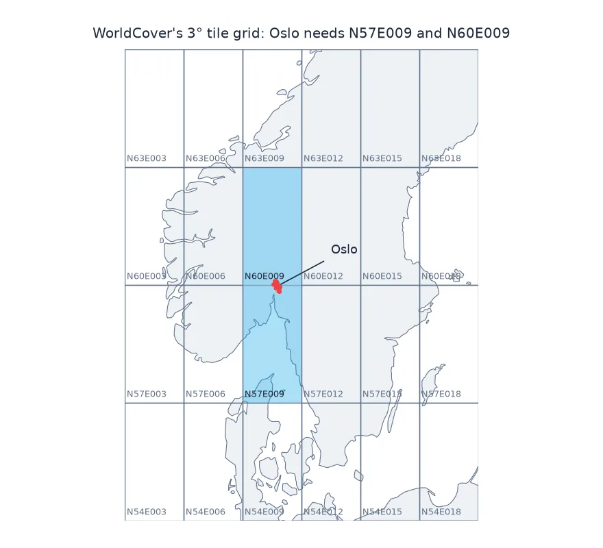
ESA WorldCover maps land cover for the whole world at 10 m, in 11 classes, for 2020 and 2021. It is published as 2,651 GeoTIFF tiles of 3° × 3° each on a public S3 bucket, every one a cloud-optimised GeoTIFF (COG). An area of interest rarely sits inside one tile, and downloading whole tiles of up to a few hundred megabytes for a city is wasteful. The tile names encode their lower-left corner, so the tiles for any area can be computed, and because the files are COGs, only the part inside the area needs to cross the network.

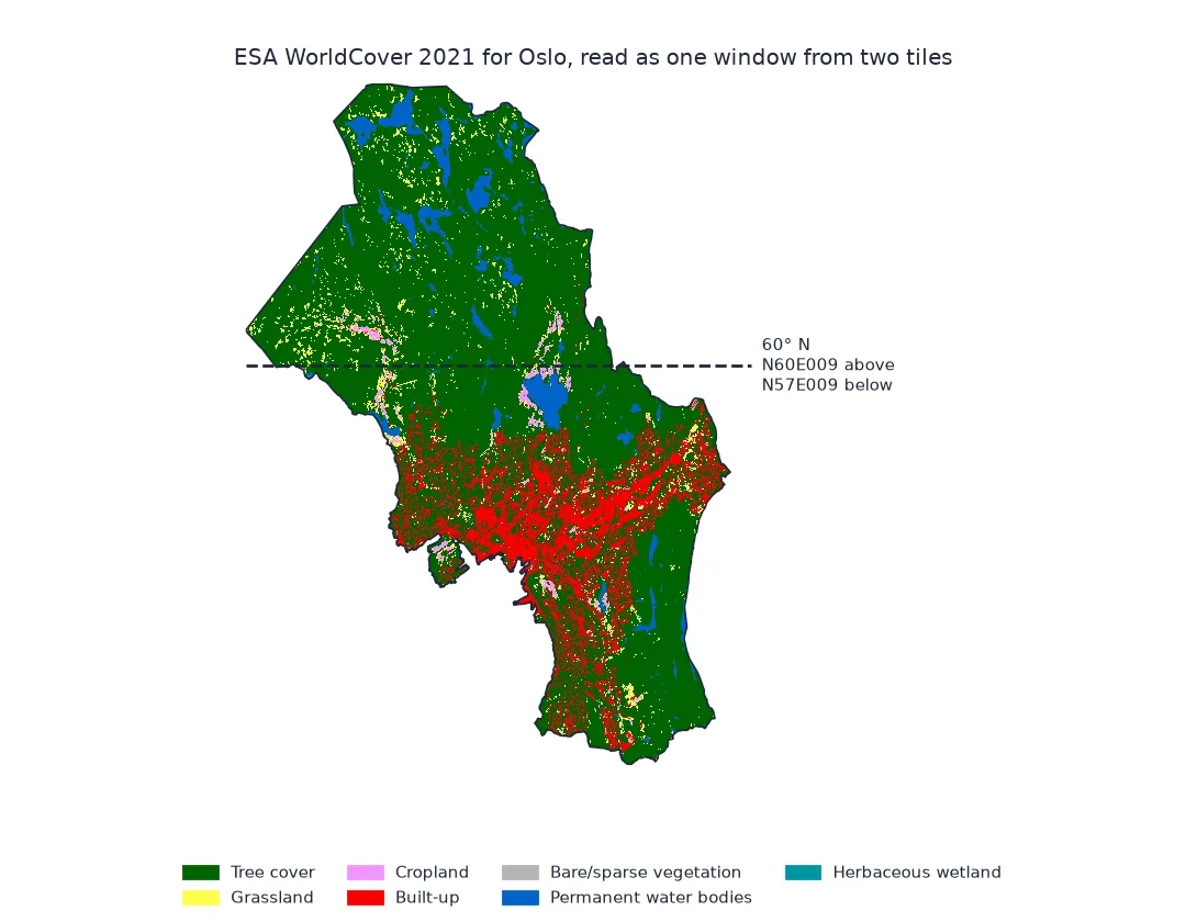
This page reads WorldCover 2021 for the municipality of Oslo, which straddles the 60° N line between two tiles, reading only the windows it needs.

Quick answer

List the tiles covering the bounds, open them over HTTP, and merge just the area's window:

def tiles_for(bounds):
    lon0, lat0, lon1, lat1 = bounds
    lats = range(int(np.floor(lat0 / 3) * 3), int(np.ceil(lat1 / 3) * 3), 3)
    lons = range(int(np.floor(lon0 / 3) * 3), int(np.ceil(lon1 / 3) * 3), 3)
    return [f"{'N' if la >= 0 else 'S'}{abs(la):02d}{'E' if lo >= 0 else 'W'}{abs(lo):03d}" for la in lats for lo in lons]

names = tiles_for(OSLO.total_bounds)
srcs = [rasterio.open(f"/vsicurl/{BUCKET}/v200/2021/map/ESA_WorldCover_10m_2021_v200_{n}_Map.tif") for n in names]
mosaic, transform = merge(srcs, bounds=tuple(OSLO.total_bounds))
print(f"tiles {names}; mosaic {mosaic.shape[2]} x {mosaic.shape[1]} pixels of {transform.a:.10f}°")

tiles ['N57E009', 'N60E009']; mosaic 5547 x 3910 pixels of 0.0000833333°

Name the tiles, read a window, mask and count

1. Name the tiles

Each tile is named after its south-west corner in whole degrees, on a 3° grid. Oslo runs from 59.81° to 60.14° N, so it needs the tile starting at 57° N and the one starting at 60° N:

for n, s in zip(names, srcs):
    b = s.bounds
    print(f"{n}: {b.left:.0f}–{b.right:.0f}° E, {b.bottom:.0f}–{b.top:.0f}° N; {s.width:,} x {s.height:,} pixels; "
          f"tiled {s.profile['blockxsize']} x {s.profile['blockysize']}, overviews {s.overviews(1)}")

N57E009: 9–12° E, 57–60° N; 36,000 x 36,000 pixels; tiled 1024 x 1024, overviews [2, 4, 8, 16, 32, 64]
N60E009: 9–12° E, 60–63° N; 36,000 x 36,000 pixels; tiled 1024 x 1024, overviews [2, 4, 8, 16, 32, 64]

2. Read only the window

A COG stores its pixels in blocks, so a reader can fetch the few blocks covering a window with HTTP range requests. GDAL does this for /vsicurl/ paths. Compare the size of the window with the size of the tiles it comes from:

sizes = {n: int(requests.head(f"{BUCKET}/v200/2021/map/ESA_WorldCover_10m_2021_v200_{n}_Map.tif", timeout=60).headers["Content-Length"]) for n in names}
print("tile sizes:", {n: f"{v / 1e6:.0f} MB" for n, v in sizes.items()})
print(f"the window holds {mosaic.size:,} pixels = {mosaic.nbytes / 1e6:.1f} MB uncompressed")

tile sizes: {'N57E009': '41 MB', 'N60E009': '83 MB'}
the window holds 21,688,770 pixels = 21.7 MB uncompressed

3. Mask to the boundary and count classes

profile = dict(driver="GTiff", height=mosaic.shape[1], width=mosaic.shape[2], count=1, dtype="uint8", crs="EPSG:4326",
               transform=transform, nodata=0, compress="deflate")
with rasterio.open("data/oslo_worldcover.tif", "w", **profile) as dst:
    dst.write(mosaic)
with rasterio.open("data/oslo_worldcover.tif") as src:
    wc = rasterio.mask.mask(src, OSLO.geometry, crop=True, nodata=0)[0][0]
v, n = np.unique(wc[wc > 0], return_counts=True)
print(pd.Series(n / n.sum() * 100, index=[WC_CLASSES[k] for k in v]).round(1).sort_values(ascending=False).to_string())

Tree cover                74.8
Built-up                  13.8
Permanent water bodies     5.7
Grassland                  4.0
Cropland                   1.5
Bare/sparse vegetation     0.1
Herbaceous wetland         0.1

These are shares of pixels. In EPSG:4326 pixels do not all cover the same area, so shares of pixels equal shares of area only where latitude barely varies, as within one city; for areas in km² see why land cover areas in degrees are wrong.

The 2020 map for the same area

The data used on this page

ESA WorldCover 10 m 2021 v200 from the public S3 bucket esa-worldcover (eu-central-1), and the municipality of Oslo from geoBoundaries Norway ADM2 (source: Geonorge, CC BY 4.0).

from pathlib import Path

import geopandas as gpd
import numpy as np
import pandas as pd
import rasterio
import rasterio.mask
import requests
from rasterio.merge import merge

Path("data").mkdir(exist_ok=True)
BUCKET = "https://esa-worldcover.s3.eu-central-1.amazonaws.com"
F = Path("data/nor_adm2.geojson")
if not F.exists():
    F.write_bytes(requests.get("https://github.com/wmgeolab/geoBoundaries/raw/9469f09/releaseData/gbOpen/NOR/ADM2/geoBoundaries-NOR-ADM2.geojson", timeout=300).content)
adm2 = gpd.read_file(F)
OSLO = adm2[adm2.shapeName.str.startswith("Oslo")]
WC_CLASSES = {10: "Tree cover", 20: "Shrubland", 30: "Grassland", 40: "Cropland", 50: "Built-up", 60: "Bare/sparse vegetation",
              70: "Snow and ice", 80: "Permanent water bodies", 90: "Herbaceous wetland", 95: "Mangroves", 100: "Moss and lichen"}
print(f"{OSLO.shapeName.iloc[0]}: bounds {OSLO.total_bounds.round(3)}")

Oslo nor: bounds [10.489 59.809 10.951 60.135]

Example 1: the 2020 map for the same area

WorldCover 2020 (v100) uses a different algorithm version, so differences from 2021 are partly method, not change:

srcs20 = [rasterio.open(f"/vsicurl/{BUCKET}/v100/2020/map/ESA_WorldCover_10m_2020_v100_{n}_Map.tif") for n in names]
m20, _ = merge(srcs20, bounds=tuple(OSLO.total_bounds))
same = (m20[0] == mosaic[0])[mosaic[0] > 0]
print(f"pixels with the same class in 2020 and 2021 within the window: {same.mean():.1%}")

pixels with the same class in 2020 and 2021 within the window: 93.2%

Why global rasters come in named tiles

Global rasters at 10 m are too large for single files: WorldCover would be terabytes. Splitting them into fixed tiles with predictable names lets any client find the files for an area without an index. Storing each tile as a COG lets the client read part of a file over plain HTTP. Together they make "the land cover of Oslo" a read of one window, not a download of two tiles of 41 and 83 MB.

WorldCover keeps the geographic grid of its source data: pixels of 1/12,000 of a degree in longitude and latitude. That is about 10 m north–south everywhere, but east–west it shrinks with the cosine of latitude, to about 4.6 m at Oslo. The map is in degrees, so anything measured in metres, such as area, needs that correction or a reprojection to an equal-area CRS.

Versions, missing tiles and merging

• Versions: 2020 is v100 and 2021 is v200, made with different algorithm versions; differences between them mix real change with method change, so do not read them as change (Example 1: 93.2% of pixels agree).
• Tiles that do not exist: open-ocean tiles are not published; skip missing names.
• Merging: rasterio.merge takes the first dataset's value where tiles overlap; WorldCover tiles abut exactly.
• Credentials: the bucket is public; set AWS_NO_SIGN_REQUEST=YES if reading through s3:// paths.
• Other products: the same tile-and-COG pattern applies to Copernicus DEM, Hansen forest change and many others.

Internal links

• Land cover products explained — WorldCover among the others
• Why are land cover areas in degrees wrong? — pixel areas at this latitude

FAQ

How do I download ESA WorldCover for an area?

Compute the 3° tile names for its bounds, open the tiles from the esa-worldcover S3 bucket with /vsicurl/ paths, and read or merge only the window you need.

What are WorldCover tile names?

ESA_WorldCover_10m_2021_v200_N60E009_Map.tif covers 60–63° N and 9–12° E: the name is the south-west corner on a 3° grid.

Do I need to download the whole tile?

No. The tiles are cloud-optimised GeoTIFFs, so GDAL fetches only the blocks covering your window.

What projection is WorldCover in?

Geographic WGS 84 (EPSG:4326), with pixels of 1/12,000 of a degree, about 10 m north–south.