How to Map Snow Cover from Sentinel-2 in Python

On this page

Problem statement

Sentinel-2 sees snow at 10–20 m every few days, fine enough to map snow patch by patch on a single mountainside. Turning a scene into a snow map takes four decisions: how to read the reflectance (the Level-2A offset changed in 2022), which index and threshold mark snow, what to do with cloud, and how to tell snow from the other bright or high-index surfaces in a mountain scene. Get any of them wrong and the map is confidently wrong.

This page maps snow over a 19 × 18 km window of Rocky Mountain National Park, Colorado, on six cloud-light dates from February to July 2024, using Sentinel-2 Level-2A from Microsoft's Planetary Computer, and saves the result as a GeoTIFF.

Quick answer

Read green, near-infrared and short-wave infrared, subtract the Level-2A offset, mask cloud with the scene classification, and call a pixel snow where NDSI exceeds 0.4 and the near infrared is bright enough to exclude water:

def snow_map(item, box):
    b = read_bands(item, ("B03", "B08", "B11", "SCL"), box)
    off = 1000 if float(item.properties["s2:processing_baseline"]) >= 4 else 0
    g, nir, swir = ((b[k] - off) / 10000 for k in ("B03", "B08", "B11"))
    ndsi = (g - swir) / (g + swir + 1e-9)
    valid = ~np.isin(b["SCL"], [0, 3, 8, 9, 10])               # no data, cloud shadow, cloud, cirrus
    return np.where(valid, ((ndsi > 0.4) & (nir > 0.11)).astype(np.uint8), 255), b["transform"], b["crs"]

snow, tr, crs = snow_map(ITEMS["20240530"], BOX)
print(f"30 May 2024: {(snow == 1).sum() / (snow != 255).sum():.0%} of cloud-free ground snow-covered; "
      f"{(snow == 255).mean():.1%} masked as cloud or shadow")

30 May 2024: 46% of cloud-free ground snow-covered; 0.8% masked as cloud or shadow

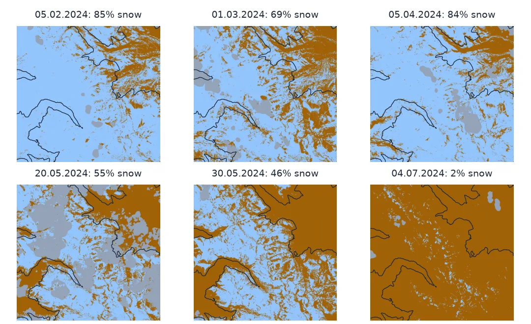
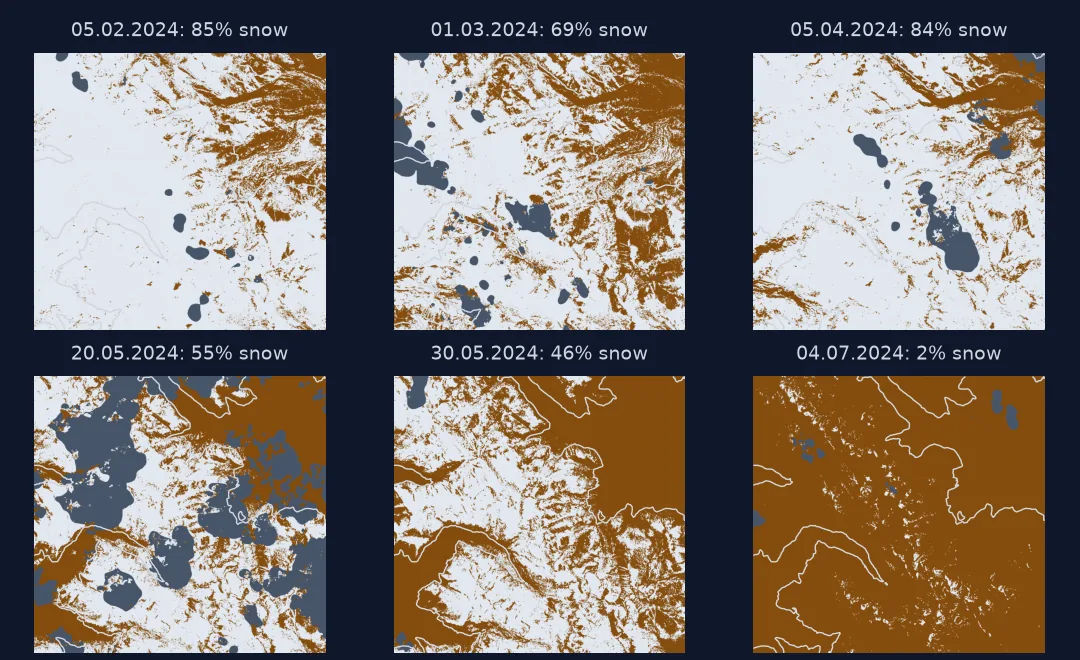
Six Sentinel-2 snow maps of a 19 by 18 km window of Rocky Mountain National Park in 2024: snow in blue covers most of the window on 5 February and 5 April, retreats to the high ground by 30 May, and is almost gone on 4 July; brown is snow-free ground, grey masked cloud, and a black line the 3,000 m contour. — NDSI > 0.4 and NIR > 0.11, SCL cloud masked. Copernicus Sentinel-2 data 2024 via Planetary Computer.

Clear scenes, right reflectance, cloud and water masks

Five steps from a scene to a snow map.

1. Find clear scenes

Search by box and date range, and filter on the scene's cloud cover. Cloud cover is for the whole 110 km tile; your window can be cloudier or clearer:

found = catalog.search(collections=["sentinel-2-l2a"], bbox=BOX, datetime="2024-02-01/2024-07-15",
                       query={"eo:cloud_cover": {"lt": 20}})
for it in sorted(found.items(), key=lambda i: i.datetime)[:9]:
    print(it.id[11:19], it.properties["s2:mgrs_tile"], round(it.properties["eo:cloud_cover"], 1))

20240205 13TDE 0.6
20240225 13TDE 0.9
20240301 13TDE 1.4
20240321 13TDE 7.2
20240405 13TDE 11.9
20240520 13TDE 16.9
20240530 13TDE 3.3
20240530 13TDE 1.1
20240704 13TDE 0.5

2. Read the right reflectance

Since processing baseline 04.00 (January 2022) Level-2A values carry an offset of 1,000. All six scenes here are baseline 05.10, so reflectance is (value − 1000) / 10,000; for scenes processed earlier the offset is zero. Read the property every time rather than assuming it.

3. Mask cloud with the scene classification

The scene classification layer (SCL) labels cloud shadow (3), medium and high cloud (8, 9) and thin cirrus (10). Masking them is crude but honest — the alternative, letting cloud through, makes it snow, because cloud and snow are both bright:

for d, it in ITEMS.items():
    s, _, _ = snow_map(it, BOX)
    print(f"{d}: masked {(s == 255).mean():5.1%}, snow {(s == 1).sum() / (s != 255).sum():5.1%} of the rest")

20240205: masked  1.5%, snow 84.5% of the rest
20240301: masked  6.8%, snow 68.7% of the rest
20240405: masked  5.0%, snow 84.3% of the rest
20240520: masked 30.2%, snow 55.4% of the rest
20240530: masked  0.8%, snow 45.7% of the rest
20240704: masked  1.2%, snow  2.3% of the rest

4. Keep water out

NDSI alone flags some lakes as snow: water can be dark in both bands. A near-infrared floor — 0.11 here, the value used by the Sen2Cor and Theia snow algorithms — removes dark water while keeping snow, which is bright in the near infrared:

b = read_bands(ITEMS["20240704"], ("B03", "B08", "B11", "SCL"), BOX)
g, nir, swir = ((b[k] - 1000) / 10000 for k in ("B03", "B08", "B11"))
ndsi = (g - swir) / (g + swir + 1e-9)
water = b["SCL"] == 6
print(f"4 July, Sen2Cor water pixels: {water.sum():,}; with NDSI > 0.4 {((ndsi > 0.4) & water).sum():,}; "
      f"after the NIR test {((ndsi > 0.4) & (nir > 0.11) & water).sum():,}")

4 July, Sen2Cor water pixels: 3,464; with NDSI > 0.4 290; after the NIR test 45

5. Save it as a GeoTIFF

One byte per pixel: 1 snow, 0 no snow, 255 masked. A colour table makes it readable in QGIS without styling:

with rasterio.open("data/snow_20240530.tif", "w", driver="GTiff", height=snow.shape[0], width=snow.shape[1], count=1,
                   dtype="uint8", crs=crs, transform=tr, nodata=255, compress="deflate") as dst:
    dst.write(snow, 1)
    dst.write_colormap(1, {0: (161, 98, 7, 255), 1: (147, 197, 253, 255)})
print(Path("data/snow_20240530.tif").stat().st_size // 1000, "kB,", crs.to_epsg(), tr.a, "m")

205 kB, 32613 10.0 m

Snow-covered area through a season

The data used on this page

Copernicus Sentinel-2 Level-2A, tile 13TDE, 5 February, 1 March, 5 April, 20 May, 30 May and 4 July 2024 (Copernicus Sentinel data 2024, processed by ESA), via Microsoft Planetary Computer.

from pathlib import Path

import numpy as np
import planetary_computer
import pystac_client
import rasterio
from rasterio.enums import Resampling
from rasterio.warp import transform_bounds
from rasterio.windows import from_bounds

Path("data").mkdir(exist_ok=True)
catalog = pystac_client.Client.open("https://planetarycomputer.microsoft.com/api/stac/v1",
                                    modifier=planetary_computer.sign_inplace)
BOX = (-105.80, 40.22, -105.58, 40.38)
IDS = ["S2A_MSIL2A_20240205T175531_R141_T13TDE_20240205T223544", "S2B_MSIL2A_20240301T175239_R141_T13TDE_20240301T231548",
       "S2A_MSIL2A_20240405T174901_R141_T13TDE_20240406T024518", "S2B_MSIL2A_20240520T174909_R141_T13TDE_20240521T001144",
       "S2B_MSIL2A_20240530T174909_R141_T13TDE_20240530T231838", "S2A_MSIL2A_20240704T174911_R141_T13TDE_20240706T011649"]
ITEMS = {i[11:19]: catalog.get_collection("sentinel-2-l2a").get_item(i) for i in IDS}

def read_bands(item, bands, box):
    """Read `bands` for `box`, 20 m bands brought to the 10 m grid by nearest neighbour."""
    out = {}
    for band in bands:
        with rasterio.open(item.assets[band].href) as src:
            w = from_bounds(*transform_bounds(4326, src.crs, *box), src.transform).round_offsets().round_lengths()
            scale = 2 if src.res[0] == 20 else 1
            out[band] = src.read(1, window=w, out_shape=(int(w.height * scale), int(w.width * scale)),
                                 resampling=Resampling.nearest).astype(float)
            if src.res[0] == 10:
                out["transform"], out["crs"] = src.window_transform(w), src.crs
    rows = min(v.shape[0] for k, v in out.items() if k in bands)
    cols = min(v.shape[1] for k, v in out.items() if k in bands)
    for band in bands:
        out[band] = out[band][:rows, :cols]
    return out

print({d: it.properties["s2:processing_baseline"] for d, it in ITEMS.items()})

{'20240205': '05.10', '20240301': '05.10', '20240405': '05.10', '20240520': '05.10', '20240530': '05.10', '20240704': '05.10'}

Example 1: what the threshold does

The snow-covered share of 30 May at different NDSI thresholds, with the near-infrared test kept:

b = read_bands(ITEMS["20240530"], ("B03", "B08", "B11", "SCL"), BOX)
g, nir, swir = ((b[k] - 1000) / 10000 for k in ("B03", "B08", "B11"))
ndsi = (g - swir) / (g + swir + 1e-9)
valid = ~np.isin(b["SCL"], [0, 3, 8, 9, 10])
for t in (0.1, 0.2, 0.3, 0.4, 0.5):
    print(f"NDSI > {t}: {((ndsi > t) & (nir > 0.11) & valid).sum() / valid.sum():.0%}")

NDSI > 0.1: 55%
NDSI > 0.2: 52%
NDSI > 0.3: 49%
NDSI > 0.4: 46%
NDSI > 0.5: 42%

Example 2: snow-covered area through the season

for d, it in ITEMS.items():
    s, tr_, _ = snow_map(it, BOX)
    print(f"{d}: {(s == 1).sum() * tr_.a ** 2 / 1e6:6.1f} km² snow seen, {(s == 255).sum() * tr_.a ** 2 / 1e6:5.1f} km² masked")

20240205:  280.6 km² snow seen,   5.2 km² masked
20240301:  216.0 km² snow seen,  22.8 km² masked
20240405:  270.0 km² snow seen,  17.0 km² masked
20240520:  130.4 km² snow seen, 101.8 km² masked
20240530:  152.6 km² snow seen,   2.9 km² masked
20240704:    7.6 km² snow seen,   3.9 km² masked

Snow area on a date with heavy masking is a lower bound; for a time series, compare shares of the cloud-free area, or fill gaps from neighbouring dates as in the MODIS time series.

A classification built on rules

A Sentinel-2 snow map is a classification built from a physical contrast. Snow is bright in green and near-infrared light and dark in the short-wave infrared, where ice absorbs; the NDSI captures that contrast in one number. Everything else in the recipe handles the exceptions: cloud, which is bright everywhere; water, which can mimic a high NDSI by being dark in both bands; and the edges of snow patches, where a pixel is part snow and part rock and the threshold decides which it becomes.

The 2024 melt season in one window.

At 10–20 m the map resolves what coarser products cannot: individual snowfields, wind-scoured ridges, gullies that hold snow into July. The price is a revisit of five days at best and cloud on many of those, which is why Sentinel-2 snow maps are often combined with daily MODIS: one for detail, the other for timing.

Processing baselines, SCL classes and band resampling

Why the NIR test belongs in the recipe.

Check s2:processing_baseline: offset 1,000 from 04.00, none before.
SCL cloud classes are 3, 8, 9 and 10; class 11 is Sen2Cor's own snow, more generous than NDSI > 0.4.
Add a NIR test to keep dark water out.
Bring 20 m bands to 10 m by nearest neighbour, or compute at 20 m throughout.
Tile cloud cover is not window cloud cover; check the SCL for your area.
Forest hides snow from above; see snow cover and NDSI explained.

Internal links

Snow cover and NDSI explained — the index in detail
How to find the snow line elevation — these maps with a DEM
NDSI snow confused with cloud or water — the failure cases
How to make a MODIS snow cover time series — daily, coarser
How to measure glacier retreat — the same index on glacier ice

FAQ

How do I map snow from Sentinel-2 in Python?

Read bands 3, 8 and 11 and the SCL from a Level-2A scene, convert to reflectance with the baseline offset, compute NDSI = (B3 − B11)/(B3 + B11), and classify snow where NDSI > 0.4 and B8 > 0.11, masking SCL cloud and shadow classes.

What threshold should I use for Sentinel-2 snow?

0.4 is the common threshold for snow-dominated pixels; lower values include patchy snow. On 30 May 2024 in this window, thresholds of 0.1, 0.4 and 0.5 gave 55%, 46% and 42% snow.

How do I remove clouds from a Sentinel-2 snow map?

Mask the scene classification classes for cloud shadow (3), cloud (8, 9) and cirrus (10). The masked area is unknown, not snow-free.

Why do lakes show up as snow?

Water can have a positive NDSI because it is dark in both bands. A minimum near-infrared reflectance removes it.