
Sea-Ice Extent vs Area Explained
On this page
Problem statement
Two numbers describe how much sea ice there is, and they are routinely confused. Extent is the total area of ocean cells holding at least 15% ice. Area is the ice itself: each cell's area multiplied by its concentration. In September 2025 the Arctic had 4.75 million km² of extent and 3.08 million km² of area — two "sizes" of the same ice that differ by half again. Quote the wrong one, compare one with the other, or compute either from the grid without knowing how its cells are shaped, and the answer is wrong by far more than the year-to-year changes it is meant to show.
This page computes both from NSIDC's monthly concentration grids for September 1985, 2012 and 2025, reproduces NSIDC's own published values, and shows the three mistakes that separate a naïve calculation from the official one.
Quick answer
Read the concentration grid, count the area of cells at or above 15% for extent, weight by concentration for area, use each cell's true area rather than its nominal 25 × 25 km, and count the unobserved disc around the pole in extent but not in area:
for ym in ("198509", "201209", "202509"):
    a = read_grid(ym)
    conc = np.where(a <= 1000, a / 1000, 0.0)                     # stored as tenths of a percent
    pole = a == POLE_HOLE
    ice = (conc >= 0.15) | pole
    extent = (CELL_KM2 * ice).sum() / 1e6
    area = (CELL_KM2 * np.where(conc >= 0.15, conc, 0)).sum() / 1e6          # the pole hole has no concentration
    print(f"{ym[:4]}: extent {extent:.2f}  area {area:.2f} million km²   NSIDC: {PUBLISHED[ym[:4]]}")
1985: extent 6.94 area 4.18 million km² NSIDC: extent 6.70, area 4.23
2012: extent 3.63 area 2.37 million km² NSIDC: extent 3.57, area 2.41
2025: extent 4.82 area 3.04 million km² NSIDC: extent 4.75, area 3.08
What the grid holds, extent as a count, area as a weight
1. Know what is in the grid
The NSIDC Sea Ice Index monthly concentration GeoTIFF is a 304 × 448 grid in the NSIDC polar stereographic projection (EPSG:3411), with 25 km nominal cells. Values 0–1000 are concentration in tenths of a percent; values above 1000 are flags:
a = read_grid("202509")
vals, counts = np.unique(a[a > 1000], return_counts=True)
print(dict(zip(vals.tolist(), counts.tolist())))
print("concentration cells:", int((a <= 1000).sum()), "of", a.size)
{2510: 96, 2530: 5052, 2540: 63212}
concentration cells: 67832 of 136192
2510 is the pole hole — the disc around the North Pole that the satellite's orbit never sees; 2530 is coast and 2540 land. Treating any of them as concentration (2510 is not 251%) breaks everything downstream.
2. Extent: a threshold count
Extent counts a cell fully once its concentration reaches 15%, and not at all below. A cell 15% covered counts as much as a cell 100% covered:
conc = np.where(a <= 1000, a / 1000, 0.0)
print(f"cells at >=15%: {(conc >= 0.15).sum():,}; of which >=90%: {(conc >= 0.9).sum():,}; 15-50%: {((conc >= 0.15) & (conc < 0.5)).sum():,}")
cells at >=15%: 7,273; of which >=90%: 735; 15-50%: 1,820
The threshold is a practical choice: passive microwave sensors cannot reliably tell thin, low-concentration ice from open water with surface melt, so extent is the more robust number from year to year.
3. Area: concentration-weighted
Area counts each cell in proportion to its ice, so a 30% cell contributes 30% of its area. It is always smaller than extent and moves more with melt ponds and weather, because surface water on the ice reads as lower concentration.
4. Cells are not all 625 km²
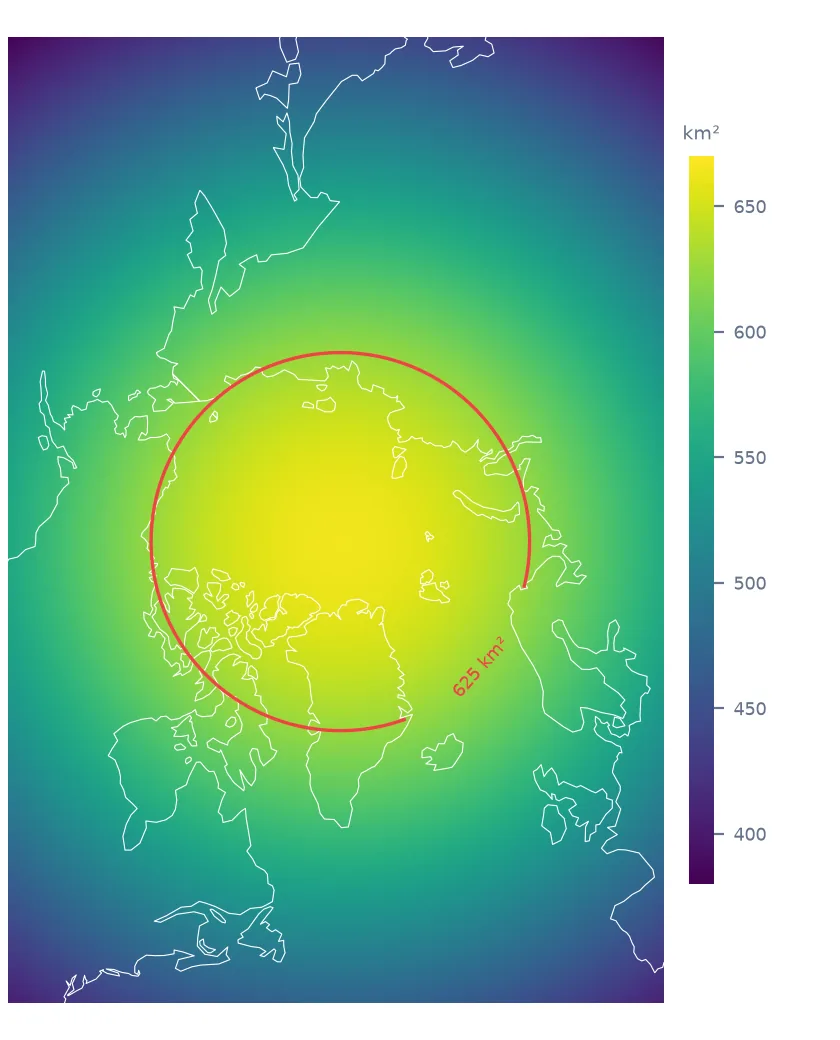
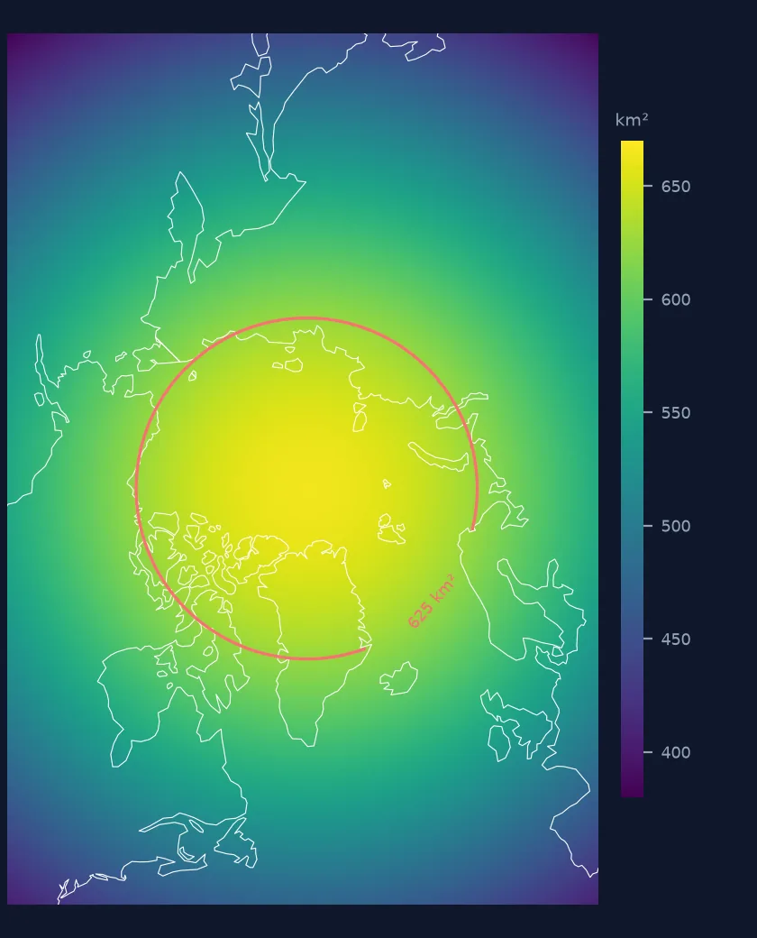
A polar stereographic grid has square cells on the map, but the projection is true to scale only at its standard parallel, 70° N. Poleward of it the map shrinks the ground, so each 25 km map cell covers more than 625 km²; further south the map enlarges the ground, and each cell covers less:
print(f"true cell area: {CELL_KM2.min():.0f} to {CELL_KM2.max():.0f} km² (nominal 625)")
ice = (conc >= 0.15)
print(f"2025 extent with nominal 625 km² cells: {ice.sum() * 625 / 1e6:.2f}; with true areas: {(CELL_KM2 * ice).sum() / 1e6:.2f} million km²")
true cell area: 383 to 664 km² (nominal 625)
2025 extent with nominal 625 km² cells: 4.55; with true areas: 4.76 million km²
NSIDC uses a separate file of true cell areas; computing them from the projection, as the setup block does, gives nearly the same thing.
5. The pole hole counts in extent
The disc the satellite cannot see is ice-covered in reality, so it belongs in extent; it has no measured concentration, so it cannot be in area. NSIDC's published figures bear that out — 1985's extent needs the hole, and 1985's area matches without it. Its size changed with the sensor, far larger in the 1980s than now:
for ym in ("198509", "201209", "202509"):
    hole = (read_grid(ym) == POLE_HOLE)
    print(f"{ym[:4]}: pole hole {(CELL_KM2 * hole).sum() / 1e6:.2f} million km²")
1985: pole hole 1.19 million km²
2012: pole hole 0.03 million km²
2025: pole hole 0.06 million km²
Leave it out of extent and 1985 loses 1.2 million km² of ice that was there, inventing a decline. This is the largest of the three mistakes. With all three handled, the grid reproduces NSIDC's published area to within 2% and its extent to within 4%; the remainder is consistent with NSIDC computing its monthly values from daily fields and its own coastline handling, which the monthly grid alone cannot reproduce.
Three mistakes, one at a time
The data used on this page
NSIDC Sea Ice Index, version 4 (G02135): monthly concentration GeoTIFFs and the monthly extent and area table for September, Northern Hemisphere, from NSIDC / NOAA. Fetterer, F., K. Knowles, W. N. Meier, M. Savoie, and A. K. Windnagel. Sea Ice Index, Version 4. NSIDC: National Snow and Ice Data Center.
from pathlib import Path

import numpy as np
import pandas as pd
import rasterio
import requests
from pyproj import Proj, Transformer

Path("data").mkdir(exist_ok=True)
UA = {"User-Agent": "spatialworkflow.io guide (https://www.spatialworkflow.io)"}
BASE = "https://noaadata.apps.nsidc.org/NOAA/G02135/north/monthly"
for ym in ("198509", "201209", "202509"):
    f = Path(f"data/N_{ym}_concentration_v4.0.tif")
    if not f.exists():
        f.write_bytes(requests.get(f"{BASE}/geotiff/09_Sep/{f.name}", headers=UA, timeout=120).content)
if not Path("data/N_09_extent_v4.0.csv").exists():
    Path("data/N_09_extent_v4.0.csv").write_bytes(requests.get(f"{BASE}/data/N_09_extent_v4.0.csv", headers=UA, timeout=120).content)

POLE_HOLE = 2510

def read_grid(ym):
    with rasterio.open(f"data/N_{ym}_concentration_v4.0.tif") as src:
        return src.read(1)

with rasterio.open("data/N_202509_concentration_v4.0.tif") as src:          # the grid is the same every month
    rows, cols = np.mgrid[0:src.height, 0:src.width]
    xs, ys = rasterio.transform.xy(src.transform, rows.ravel(), cols.ravel())
    lon, lat = Transformer.from_crs(src.crs, 4326, always_xy=True).transform(np.array(xs), np.array(ys))
    CELL_KM2 = (625 / Proj(src.crs).get_factors(lon, lat).areal_scale).reshape(src.shape)  # true area of each cell

tab = pd.read_csv("data/N_09_extent_v4.0.csv", skipinitialspace=True)
tab.columns = tab.columns.str.strip()
PUBLISHED = {str(r.year): f"extent {r.extent:.2f}, area {r.area:.2f}" for r in tab.itertuples() if r.year in (1985, 2012, 2025)}
print(PUBLISHED)
{'1985': 'extent 6.70, area 4.23', '2012': 'extent 3.57, area 2.41', '2025': 'extent 4.75, area 3.08'}
Example 1: the three mistakes, one at a time
Start naïve and fix one thing at a time, for September 1985, when the pole hole was largest:
a = read_grid("198509")
conc = np.where(a <= 1000, a / 1000, 0.0)
steps = {
    "625 km² cells, no pole hole":   ((conc >= 0.15) * 625).sum(),
    "true cell areas, no pole hole": ((conc >= 0.15) * CELL_KM2).sum(),
    "true cell areas + pole hole":   (((conc >= 0.15) | (a == POLE_HOLE)) * CELL_KM2).sum(),
}
area = {"area, pole hole as 100% ice": ((np.where(conc >= 0.15, conc, 0) + (a == POLE_HOLE)) * CELL_KM2).sum(),
        "area, pole hole left out":    (np.where(conc >= 0.15, conc, 0) * CELL_KM2).sum()}
steps.update(area)
for k, v in steps.items():
    print(f"{k:32} {v / 1e6:.2f} million km²")
print("NSIDC published:", PUBLISHED["1985"])
625 km² cells, no pole hole 5.54 million km²
true cell areas, no pole hole 5.74 million km²
true cell areas + pole hole 6.94 million km²
area, pole hole as 100% ice 5.37 million km²
area, pole hole left out 4.18 million km²
NSIDC published: extent 6.70, area 4.23
Example 2: extent and area tell different stories
The ratio of area to extent — how compact the pack is — changes between years:
for r in tab[tab.year.isin([1985, 2007, 2012, 2020, 2025])].itertuples():
    print(f"{r.year}: extent {r.extent:.2f}, area {r.area:.2f}, area/extent {r.area / r.extent:.2f}")
1985: extent 6.70, area 4.23, area/extent 0.63
2007: extent 4.27, area 2.82, area/extent 0.66
2012: extent 3.57, area 2.41, area/extent 0.68
2020: extent 4.00, area 2.83, area/extent 0.71
2025: extent 4.75, area 3.08, area/extent 0.65
A loose, broken pack has a large extent and a small area; a compact one has the two close together. A year can rank differently by extent and by area, which is why a "record" should always say which.
Sea ice is not a solid sheet
Sea ice is not a solid sheet with an edge; it is a field of floes of varying concentration, from scattered pieces at the margin to almost unbroken pack at the centre. A satellite passive microwave sensor sees a footprint tens of kilometres across and estimates the fraction of it covered by ice. Turning that field into one number requires a choice, and the two standard choices give the two numbers.
Extent asks "where is there meaningful ice?" and draws a line at 15%. It is insensitive to the hardest part of the measurement — telling 40% ice from 60% when the surface is wet — so it is the preferred long-term indicator. Area asks "how much ice is there?" and is closer to the physical quantity, but carries more of the sensor's uncertainty. Both depend on how the grid's cells map to the ground and on what is done with the unobserved pole, which are bookkeeping, not science — and that bookkeeping is where most homemade numbers go wrong.
Flags, true cell areas and the pole hole
- Values above 1000 are flags, not concentrations: pole hole, coast, land.
- Polar stereographic cells vary in true area by almost a factor of two across the grid.
- The pole hole shrank with newer sensors; count it in extent, or the trend is wrong.
- Extent and area rank years differently; say which you mean.
- Monthly grids average daily concentration, so a monthly extent from the grid is not the mean of daily extents exactly.
- Antarctic grids use EPSG:3412 and the same flags, without a pole hole problem.
Internal links
- How to analyse a sea-ice extent time series — the daily record
- How to map sea-ice concentration — drawing these grids
- Polar stereographic projections explained — why cells differ in size
- Sea-ice extent numbers disagree — when two sources do not match
- Snow cover and NDSI explained — the land side of the cryosphere
FAQ
What is the difference between sea-ice extent and sea-ice area?
Extent is the total area of grid cells with at least 15% ice concentration; area is the sum of each cell's area times its concentration. Area is always the smaller number.
Why is the 15% threshold used for sea-ice extent?
Below about 15%, passive microwave estimates are unreliable and easily confused with open water affected by weather; the threshold makes extent a robust indicator over decades.
What is the pole hole in sea-ice data?
The region around the North Pole that the satellite's orbit does not cover. It is assumed to be ice-covered and counted in extent; having no measured concentration, it is not in area. Its size depends on the sensor: 1.19 million km² in 1985, 0.06 million km² in 2025.
How do I compute sea-ice extent from a concentration grid?
Count cells at or above 15% plus the pole hole, multiply by each cell's true area — not the nominal 625 km² — and sum. That reproduced NSIDC's September values here to within 4%.