
How to Make a MODIS Snow Cover Time Series in Python
On this page
Problem statement
MODIS has mapped snow cover every day since 2000 at 500 m resolution, and its daily product, MOD10A1, is the standard way to follow a snowpack across a whole mountain range rather than at a handful of stations. Turning it into a time series runs into three problems at once: clouds hide the ground on about half the days, the data come in a sinusoidal projection that no other dataset uses, and the snow value is a normalised difference index rather than a yes or no. Ignore them and a "snow-covered area" curve becomes a cloud-cover curve.
This page builds the water-year 2024 snow-cover record for a 34 × 44 km box over Rocky Mountain National Park, Colorado, from MOD10A1 version 6.1 on Microsoft's Planetary Computer, fills the cloud gaps, and checks the result against seven SNOTEL stations inside the box.
Quick answer
Search the STAC catalogue, read just your window from each daily file, treat values 0–100 as observations and everything above as no data, call NDSI ≥ 10 snow, and carry each pixel's last clear observation forward a few days:
items = [i for i in catalog.search(collections=["modis-10A1-061"], bbox=BOX, datetime="2023-10-01/2024-09-30").items()
         if i.id.startswith("MOD10A1") and ".h09v04." in i.id]
stack, dates = read_window(items, BOX)                  # (days, rows, cols) of NDSI_Snow_Cover, one per date
valid = stack <= 100                                     # 0-100: NDSI x 100; 200+: cloud, night, water, fill
state = np.where(valid, (stack >= 10).astype(float), np.nan)
filled = pd.DataFrame(state.reshape(len(dates), -1), index=dates).ffill(limit=5).to_numpy().reshape(state.shape)
print(f"{len(dates)} days; clear {valid.mean():.0%} of pixel-days; unknown after filling {np.isnan(filled).mean():.0%}")
366 days; clear 51% of pixel-days; unknown after filling 6%
Find tiles, read a window, decode, fill gaps
1. Find the tiles
MODIS land products are cut into 10° tiles on a sinusoidal grid, named by horizontal and vertical index. The park is in tile h09v04; the tile boundary runs along 40° N, so a box that crossed it would need two tiles per day. The collection holds both Terra (MOD) and Aqua (MYD) files; Terra passes in the morning, before afternoon cloud builds, so use it alone or Terra first:
ids = [i.id for i in catalog.search(collections=["modis-10A1-061"], bbox=BOX, datetime="2024-03-05/2024-03-05").items()]
print(ids)
print(len(items), "Terra files for water year 2024 in tile h09v04")
['MYD10A1.A2024065.h09v04.061.2024067050202', 'MOD10A1.A2024065.h09v04.061.2024067050143']
370 Terra files for water year 2024 in tile h09v04
2. Read a window, not the tile
Each tile is 2400 × 2400 pixels; the box is a few thousand of them. A Cloud-Optimised GeoTIFF read with a window fetches only the blocks needed — about a second per day. The window is a rectangle in the sinusoidal projection, so it covers a little more than the longitude–latitude box:
with rasterio.open(items[0].assets["NDSI_Snow_Cover"].href) as src:
    print(src.crs.to_proj4() if src.crs.to_epsg() is None else src.crs, round(src.res[0], 1), "m pixels")
print(stack.shape, "window per day")
+proj=sinu +lon_0=0 +x_0=0 +y_0=0 +R=6371007.181 +units=m +no_defs=True 463.3 m pixels
(366, 96, 188) window per day
3. Read the codes
Values 0–100 are the NDSI multiplied by 100. Everything above 100 is a code:
codes = {200: "missing", 201: "no decision", 211: "night", 237: "inland water", 239: "ocean",
         250: "cloud", 254: "detector saturated", 255: "fill"}
u, c = np.unique(stack[stack > 100], return_counts=True)
print({codes.get(int(k), int(k)): f"{n / stack.size:.1%}" for k, n in zip(u, c)})
{'missing': '0.0%', 'no decision': '0.4%', 'inland water': '0.4%', 'cloud': '47.6%', 'fill': '0.5%'}
Cloud is by far the largest. Every day's clear area is different, so a daily snow-covered percentage must be computed over that day's clear pixels only — and days with little clear sky give little information.
4. Fill the gaps
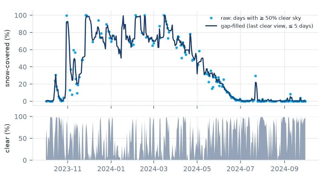
Snow cover changes slowly compared with the weather. Carrying each pixel's last clear observation forward for up to five days fills most cloudy days with a value that is very likely still right:
raw = (stack >= 10).sum((1, 2)) / np.maximum(valid.sum((1, 2)), 1)
clear_share = valid.mean((1, 2))
print(f"days with less than 10% clear sky: {(clear_share < 0.1).sum()}; "
      f"snow-covered share, monthly mean of gap-filled pixels:")
print(pd.Series(np.nanmean(filled, axis=(1, 2)), index=dates).resample("MS").mean().round(2).to_string())
days with less than 10% clear sky: 75; snow-covered share, monthly mean of gap-filled pixels:
2023-10-01 0.11
2023-11-01 0.52
2023-12-01 0.79
2024-01-01 0.73
2024-02-01 0.83
2024-03-01 0.78
2024-04-01 0.62
2024-05-01 0.35
2024-06-01 0.10
2024-07-01 0.03
2024-08-01 0.01
2024-09-01 0.01
Freq: MS
5. Check against the ground
Seven SNOTEL stations stand inside the box. For each, compare the day its snow pillow first read zero after the peak with the day its MODIS pixel first went snow-free:
for name, elev, ground, sat in station_check(filled, dates):
    print(f"{name:16} {elev:5.0f} m   SNOTEL {ground:%d %b}   MODIS {sat:%d %b}   {(sat - ground).days:+3d} days")
Copeland Lake 2612 m SNOTEL 13 Apr MODIS 09 Apr -4 days
Phantom Valley 2752 m SNOTEL 21 May MODIS 16 May -5 days
Wild Basin 2868 m SNOTEL 04 Jun MODIS 13 May -22 days
Bear Lake 2893 m SNOTEL 05 Jun MODIS 23 May -13 days
Sawtooth 2938 m SNOTEL 17 Jun MODIS 28 May -20 days
Lake Irene 3255 m SNOTEL 10 Jun MODIS 07 Jun -3 days
Willow Park 3264 m SNOTEL 10 Jun MODIS 11 Jun +1 days
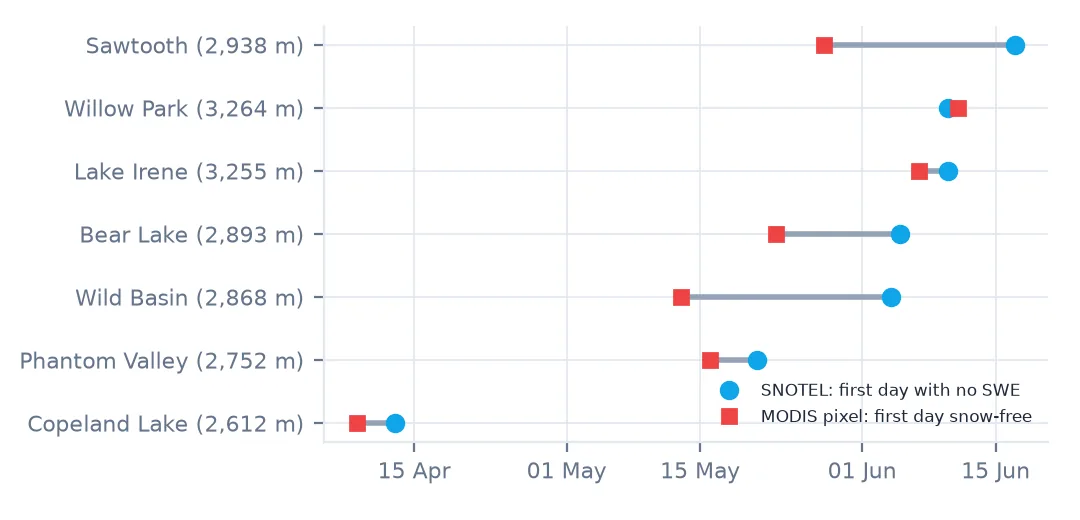
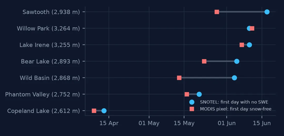
MODIS called the snow gone earlier than the ground did, by a median of five days and by up to three weeks at three stations. Those three — Wild Basin, Sawtooth and Bear Lake — sit in forest; a 500 m pixel there sees mostly canopy, and once the snow on open ground and on the trees has gone, the snow beneath the trees is invisible from orbit. The two highest, open stations agree within three days.
Snow-cover duration against elevation
The data used on this page
MODIS/Terra Snow Cover Daily L3 Global 500m SIN Grid, Version 61 (MOD10A1.061), Hall, D. K. and G. A. Riggs, NASA NSIDC DAAC, via Microsoft Planetary Computer; NRCS SNOTEL daily SWE from the AWDB REST API; Copernicus DEM GLO-30 (© DLR e.V. 2010–2014 and © Airbus Defence and Space GmbH 2014–2018, provided under COPERNICUS by the European Union and ESA) from the AWS Open Data registry. Water year 2024: 1 October 2023 to 30 September 2024.
import numpy as np
import pandas as pd
import planetary_computer
import pystac_client
import rasterio
import requests
from pyproj import Transformer
from rasterio.warp import Resampling, reproject, transform_bounds
from rasterio.windows import from_bounds

BOX = (-105.9, 40.1, -105.5, 40.5)                        # Rocky Mountain National Park, lon/lat
catalog = pystac_client.Client.open("https://planetarycomputer.microsoft.com/api/stac/v1",
                                    modifier=planetary_computer.sign_inplace)
AWDB = "https://wcc.sc.egov.usda.gov/awdbRestApi/services/v1"
STATIONS = ["322:CO:SNTL", "1042:CO:SNTL", "412:CO:SNTL", "565:CO:SNTL", "688:CO:SNTL", "1251:CO:SNTL", "870:CO:SNTL"]

def read_window(items, box):
    """Read the same window of NDSI_Snow_Cover from each item; keep the last file for each date."""
    by_date = {}
    for it in sorted(items, key=lambda i: i.id):
        href = planetary_computer.sign(it).assets["NDSI_Snow_Cover"].href
        with rasterio.open(href) as src:
            w = from_bounds(*transform_bounds("EPSG:4326", src.crs, *box), src.transform).round_offsets().round_lengths()
            by_date[it.properties["start_datetime"][:10]] = src.read(1, window=w)
            read_window.transform, read_window.crs = src.window_transform(w), src.crs
    dates = pd.to_datetime(sorted(by_date))
    return np.array([by_date[d.strftime("%Y-%m-%d")] for d in dates]), dates

def station_check(filled, dates):
    meta = requests.get(f"{AWDB}/stations?stationTriplets={','.join(STATIONS)}", timeout=60).json()
    to_sin = Transformer.from_crs(4326, read_window.crs, always_xy=True)
    out = []
    for m in sorted(meta, key=lambda m: m["elevation"]):
        col, row = ~read_window.transform * to_sin.transform(m["longitude"], m["latitude"])
        v = requests.get(f"{AWDB}/data?stationTriplets={m['stationTriplet']}&elements=WTEQ&duration=DAILY"
                         "&beginDate=2023-10-01&endDate=2024-09-30", timeout=60).json()[0]["data"][0]["values"]
        swe = pd.Series([x["value"] for x in v], index=pd.to_datetime([x["date"] for x in v]))
        peak = swe.idxmax()
        ground = swe[peak:][swe[peak:] <= 0].index.min()
        pix = pd.Series(filled[:, int(row), int(col)], index=dates)[peak:]
        out.append((m["name"], m["elevation"] * 0.3048, ground, pix[pix == 0].index.min()))
    return out

print(len(STATIONS), "SNOTEL stations in the box")
7 SNOTEL stations in the box
Example 1: snow-cover duration against elevation
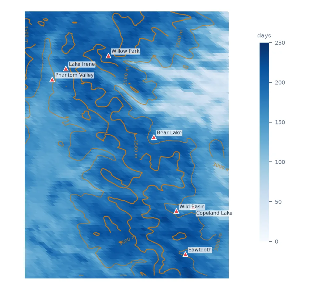
Snow-covered days per pixel, against elevation from the Copernicus DEM resampled to the MODIS grid:
dem = np.zeros(stack.shape[1:], np.float32)
dem_url = ("https://copernicus-dem-30m.s3.amazonaws.com/Copernicus_DSM_COG_10_N40_00_W106_00_DEM/"
           "Copernicus_DSM_COG_10_N40_00_W106_00_DEM.tif")
with rasterio.open(dem_url) as src:
    reproject(src.read(1), dem, src_transform=src.transform, src_crs=src.crs,
              dst_transform=read_window.transform, dst_crs=read_window.crs, resampling=Resampling.average)
days = np.nansum(filled == 1, axis=0)
for lo in range(2400, 3800, 200):
    m = (dem >= lo) & (dem < lo + 200)
    print(f"{lo}-{lo + 200} m: {m.sum():5d} pixels, median {np.median(days[m]):.0f} snow days")
2400-2600 m: 2039 pixels, median 118 snow days
2600-2800 m: 1753 pixels, median 139 snow days
2800-3000 m: 1349 pixels, median 160 snow days
3000-3200 m: 1488 pixels, median 180 snow days
3200-3400 m: 1610 pixels, median 197 snow days
3400-3600 m: 1247 pixels, median 203 snow days
3600-3800 m: 497 pixels, median 203 snow days
Duration climbs steeply up to about 3,300 m and then flattens: above that, almost every pixel holds snow for the whole season the satellite can see, and the length of the season is limited by the calendar rather than the elevation.
Example 2: Terra and Aqua on the same day
Aqua passes about three hours after Terra. Comparing clear-sky shares for the same dates shows why Terra is the first choice:
aqua = [i for i in catalog.search(collections=["modis-10A1-061"], bbox=BOX, datetime="2024-01-01/2024-01-31").items()
        if i.id.startswith("MYD10A1") and ".h09v04." in i.id]
a_stack, a_dates = read_window(aqua, BOX)
t_clear = pd.Series(valid.mean((1, 2)), index=dates).loc["2024-01"]
a_clear = pd.Series((a_stack <= 100).mean((1, 2)), index=a_dates)
print(f"January 2024 clear-sky share: Terra {t_clear.mean():.0%}, Aqua {a_clear.mean():.0%}")
January 2024 clear-sky share: Terra 31%, Aqua 27%
Codes, not just snow and no snow
MOD10A1 does not deliver "snow" and "no snow". It delivers the Normalised Difference Snow Index — the contrast between visible and short-wave infrared reflectance, high for snow because snow is bright in the visible and dark in the infrared — scaled by 100, with codes for everything the algorithm could not judge. Turning that into snow cover is the user's decision: NDSI 0.1 is the threshold the product's own documentation suggests for "any snow" in a pixel, and it is the one used here.
Cloud is the central problem. On a typical day half the box is unseen, and the unseen half is not random — storms bring cloud and new snow together. A daily percentage over clear pixels alone swings with the weather; filling each pixel from its own recent past uses the fact that snow cover persists for days, and limiting the fill to five days stops a single early-season observation from being carried through a storm.
The ground check is what makes the series usable. At open, high sites MODIS and the snow pillows agreed on melt-out within a few days; under forest MODIS ran up to three weeks early. That is the well-known canopy limitation of optical snow mapping, measured here rather than assumed — and a reason to quote satellite melt-out dates for forested areas with care.
Codes above 100, sinusoidal tiles and forest
- Values above 100 are codes, never snow fractions; mask them first.
- Sinusoidal tiles meet along 10° lines; a box crossing one needs two tiles a day.
- Duplicate dates occur when a file was reprocessed; keep one per date.
- Terra before Aqua for fewer clouds over mountains.
- Forest hides snow from above; expect early melt-out under canopy.
- The threshold is a choice. NDSI ≥ 10 counts thin and partial snow; a higher threshold shortens the season.
Internal links
- Snow cover and NDSI explained — what the index measures
- NDSI snow confused with cloud or water — when the index misleads
- MODIS sinusoidal tiles do not line up — the projection
- How to analyse SNOTEL snow water equivalent — the ground truth
- How to find snowmelt timing — melt-out from stations and satellites
FAQ
How do I get MODIS snow cover data in Python?
Search the modis-10A1-061 collection on Microsoft Planetary Computer with pystac-client, sign the items with planetary_computer, and read a window of the NDSI_Snow_Cover asset with rasterio.
What do the values in MOD10A1 NDSI_Snow_Cover mean?
0–100 is the NDSI × 100 for clear land pixels; 200 and above are codes such as 250 for cloud, 237 for inland water and 211 for night.
How do I deal with clouds in MODIS snow data?
Compute daily statistics over clear pixels only, and fill each pixel's cloudy days from its most recent clear observation for a limited number of days.
How accurate is MODIS snow melt-out?
At seven SNOTEL stations in Rocky Mountain National Park in 2024, MODIS melt-out was a median of five days early; at forested stations up to three weeks early, at open high-elevation stations within three days.