How to Find the Snow Line Elevation in Python

Problem statement

The snow line — the elevation above which the ground is mostly snow-covered — is one of the simplest ways to describe a mountain snowpack, and it moves through the year like a tide. Measuring it needs a snow map and an elevation model on the same grid, and a definition: the elevation where half the ground is snow-covered, the lowest elevation with any snow, or the point where snow cover becomes continuous. Each gives a different number, and mountain terrain — steep rock that sheds snow, shaded gullies that keep it — makes the curve far from tidy.

This page derives the snow line for a window of Rocky Mountain National Park, Colorado, on six dates in 2024 from Sentinel-2 snow maps and the Copernicus 30 m DEM, and compares definitions.

Quick answer

Bin the cloud-free pixels by elevation, compute the snow-covered share of each band, and take the lowest band above which every band stays at least half snow-covered:

bands = np.arange(2400, 4300, 100)
def snow_line(snow, valid, dem, top=3600, share=0.5):
    f = pd.Series({lo: snow[valid & (dem >= lo) & (dem < lo + 100)].mean()
                   for lo in bands if (valid & (dem >= lo) & (dem < lo + 100)).sum() > 200})
    upto = f[f.index < top]
    above = [lo for lo in upto.index if (upto[upto.index >= lo] >= share).all()]
    return (min(above) if above else None), f

for d in DATES:
    line, _ = snow_line(*SNOW[d], DEM)
    print(f"{d}: snow line {line if line else 'none (snow below 50% everywhere)'} m")

20240205: snow line 2600 m
20240301: snow line 2600 m
20240405: snow line 2600 m
20240520: snow line 3100 m
20240530: snow line 3200 m
20240704: snow line none (snow below 50% everywhere) m

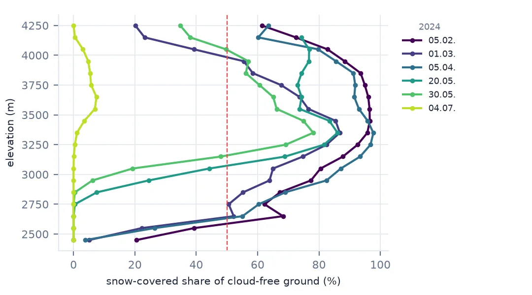
DEM on the snow grid, share by band, read the curve

1. Put the DEM on the snow map's grid

The snow map is a 10 m Sentinel-2 grid in UTM zone 13N; the Copernicus DEM is a 30 m grid in degrees. Reproject the DEM onto the snow grid with bilinear resampling so each snow pixel has an elevation:

print(DEM.shape, f"elevation {DEM.min():.0f}-{DEM.max():.0f} m;", "snow grid", SNOW["20240530"][0].shape)

(1790, 1884) elevation 2422-4341 m; snow grid (1790, 1884)

2. Compute snow share by band

Count only cloud-free pixels, and skip bands with too few of them to mean anything:

_, f = snow_line(*SNOW["20240530"], DEM)
print((f * 100).round().astype(int).to_string())

2400     0
2500     0
2600     0
2700     0
2800     0
2900     6
3000    19
3100    48
3200    69
3300    78
3400    75
3500    66
3600    65
3700    61
3800    56
3900    57
4000    50
4100    38
4200    35

3. Read the curve

Below the snow line the share drops quickly to zero; above it, it does not reach 100%. The highest bands in this window are the cliffs and rock ridges of Longs Peak and the Continental Divide, which shed snow even in midwinter — so a definition that asks for complete snow cover would put the snow line at the summit, or nowhere. Limiting the test to bands below 3,600 m keeps the definition about the snowpack, not the cliffs.

4. Compare definitions

for d in DATES:
    snow, valid = SNOW[d]
    s50, f = snow_line(snow, valid, DEM)
    s25, _ = snow_line(snow, valid, DEM, share=0.25)
    lowest = DEM[snow & valid].min() if (snow & valid).any() else np.nan
    print(f"{d}: 50% line {s50}, 25% line {s25}, lowest snow pixel {lowest:.0f} m")

20240205: 50% line 2600, 25% line 2500, lowest snow pixel 2423 m
20240301: 50% line 2600, 25% line 2600, lowest snow pixel 2427 m
20240405: 50% line 2600, 25% line 2500, lowest snow pixel 2441 m
20240520: 50% line 3100, 25% line 3000, lowest snow pixel 2611 m
20240530: 50% line 3200, 25% line 3100, lowest snow pixel 2761 m
20240704: 50% line None, 25% line None, lowest snow pixel 2763 m

The lowest snow pixel is almost meaningless — a single drift in a shaded gully. The 50% and 25% lines move together through the season and are the useful pair: one marks where snow dominates, the other where it is still common.

5. Follow it through the season

From February to April the snow line sat at the bottom of the window, around 2,600 m; by late May it had risen to about 3,100–3,200 m; by 4 July no band below 3,600 m was even a quarter snow-covered.

Aspect and the snow line as a contour

The data used on this page

Copernicus Sentinel-2 Level-2A, tile 13TDE, six dates in 2024 (Copernicus Sentinel data 2024, processed by ESA) via Microsoft Planetary Computer; Copernicus DEM GLO-30 (© DLR e.V. 2010–2014 and © Airbus Defence and Space GmbH 2014–2018, provided under COPERNICUS by the European Union and ESA) from the AWS Open Data registry.

import numpy as np
import pandas as pd
import planetary_computer
import pystac_client
import rasterio
from rasterio.enums import Resampling
from rasterio.warp import reproject, transform_bounds
from rasterio.windows import from_bounds

catalog = pystac_client.Client.open("https://planetarycomputer.microsoft.com/api/stac/v1",
                                    modifier=planetary_computer.sign_inplace)
BOX = (-105.80, 40.22, -105.58, 40.38)
IDS = ["S2A_MSIL2A_20240205T175531_R141_T13TDE_20240205T223544", "S2B_MSIL2A_20240301T175239_R141_T13TDE_20240301T231548",
       "S2A_MSIL2A_20240405T174901_R141_T13TDE_20240406T024518", "S2B_MSIL2A_20240520T174909_R141_T13TDE_20240521T001144",
       "S2B_MSIL2A_20240530T174909_R141_T13TDE_20240530T231838", "S2A_MSIL2A_20240704T174911_R141_T13TDE_20240706T011649"]
DATES = [i[11:19] for i in IDS]
SNOW = {}
for iid in IDS:
    item = catalog.get_collection("sentinel-2-l2a").get_item(iid)
    off = 1000 if float(item.properties["s2:processing_baseline"]) >= 4 else 0
    b = {}
    for band in ("B03", "B08", "B11", "SCL"):
        with rasterio.open(item.assets[band].href) as src:
            w = from_bounds(*transform_bounds(4326, src.crs, *BOX), src.transform).round_offsets().round_lengths()
            sc = 2 if src.res[0] == 20 else 1
            b[band] = src.read(1, window=w, out_shape=(int(w.height * sc), int(w.width * sc)),
                               resampling=Resampling.nearest).astype(float)
            if src.res[0] == 10:
                TR, CRS_ = src.window_transform(w), src.crs
    r, c = min(v.shape[0] for v in b.values()), min(v.shape[1] for v in b.values())
    g, nir, sw = ((b[k][:r, :c] - off) / 1e4 for k in ("B03", "B08", "B11"))
    ndsi = (g - sw) / (g + sw + 1e-9)
    valid = ~np.isin(b["SCL"][:r, :c], [0, 3, 8, 9, 10])
    SNOW[iid[11:19]] = ((ndsi > 0.4) & (nir > 0.11) & valid, valid)
DEM = np.zeros((r, c), np.float32)
with rasterio.open("https://copernicus-dem-30m.s3.amazonaws.com/Copernicus_DSM_COG_10_N40_00_W106_00_DEM/"
                   "Copernicus_DSM_COG_10_N40_00_W106_00_DEM.tif") as src:
    reproject(src.read(1), DEM, src_transform=src.transform, src_crs=src.crs, dst_transform=TR, dst_crs=CRS_,
              resampling=Resampling.bilinear)
print(len(SNOW), "snow maps,", DEM.shape)

6 snow maps, (1790, 1884)

Example 1: aspect matters

North-facing slopes keep snow longer than south-facing ones. Splitting 30 May by aspect:

gy, gx = np.gradient(DEM, 10)
aspect = (np.degrees(np.arctan2(-gx, gy)) + 360) % 360        # 0 = north-facing, clockwise
snow, valid = SNOW["20240530"]
for name, sel in (("north-facing (315-45)", (aspect >= 315) | (aspect < 45)), ("south-facing (135-225)", (aspect >= 135) & (aspect < 225))):
    line, _ = snow_line(snow, valid & sel, DEM)
    print(f"{name:24} snow line {line} m")

north-facing (315-45)    snow line 3100 m
south-facing (135-225)   snow line 3200 m

Example 2: the snow line as a contour

A snow line can be drawn on a map as the contour of the DEM at its elevation, for comparison with the snow map itself:

line, _ = snow_line(*SNOW["20240530"], DEM)
above = DEM >= line
snow, valid = SNOW["20240530"]
print(f"above {line} m: {(snow & above).sum() / (valid & above).sum():.0%} snow; below: {(snow & ~above).sum() / (valid & ~above).sum():.0%} snow")

above 3200 m: 69% snow; below: 15% snow

What a snow line summarises

A snow line summarises a snow map in one number by asking how snow cover depends on elevation. Because temperature falls with height, snow cover usually rises steeply over a few hundred metres and then levels off, and the elevation of that rise is the snow line. Its seasonal climb, from the valley floors in winter to the high ridges in summer, is one of the clearest signals in mountain snow data.

The definition decides the number. A 50% threshold marks where snow dominates; 25% where it is still frequent; any-snow is driven by isolated drifts and is not worth reporting. Terrain complicates every version: steep rock above the snowpack lowers the snow share at the top of the curve, shaded gullies push snow far below the line, and aspect shifts the line by a band or more between north and south slopes. Stating the threshold, the elevation range and the masking alongside the number is what makes snow lines comparable between dates and places.

Cloud-free pixels, sparse bands and forest

• Use only cloud-free pixels in each band.
• Skip bands with few pixels; 200 at 10 m is 0.02 km².
• Cap the elevation range below cliffs that never hold snow, or the line runs to the summit.
• Aspect shifts the line; report it separately when it matters.
• Forest hides snow, lowering the apparent share in forested bands.
• DEM resolution matters less than you think: 30 m bilinear onto 10 m is fine for 100 m bands.

Internal links

• How to map snow cover from Sentinel-2 — the snow maps used here
• Snow cover and NDSI explained — the index behind them
• How to compute glacier hypsometry from a DEM — area by elevation for glaciers
• How to find snowmelt timing — when each band melts out
• How to make a MODIS snow cover time series — duration by elevation

FAQ

What is the snow line?

The elevation above which the ground is mostly snow-covered — commonly defined as where at least half of each elevation band is snow.

How do I calculate snow line elevation from satellite data?

Reproject a DEM onto the snow map grid, compute the snow-covered share of cloud-free pixels in each elevation band, and find the lowest band above which the share stays at or above your threshold.

How did the snow line change in Rocky Mountain National Park in 2024?

In this window it stayed near 2,600 m from February to early April, rose to about 3,100–3,200 m by late May, and by early July no band below 3,600 m was a quarter snow-covered.

Why doesn't snow cover reach 100% at high elevation?

Steep rock faces and wind-scoured ridges shed snow. Above about 4,000 m in this window, snow share fell in every season.