Polar Stereographic Projections Explained

Problem statement

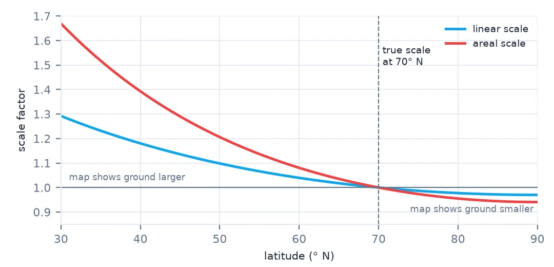
A polar stereographic projection keeps shapes true and gives up area. On NSIDC's north polar grid a 25 km cell is exactly 625 km² of ground only at 70°N, the latitude of true scale; at the pole the same cell covers 664 km², and at 50°N 518 km². That is why the projection is the standard for sea ice, ice sheets and snow — the whole polar ocean fits one square with north towards the centre — and why a total summed cell by cell, or a grid drawn as if it were latitude and longitude, comes out wrong.

This page measures the NSIDC north polar stereographic grid (EPSG:3411) with pyproj: how its scale changes with latitude, how much ground a nominal 25 km cell really covers, what that does to a sea-ice total, and when an equal-area grid is the better choice.

Quick answer

Polar stereographic is conformal — true to shape — and true to scale only at one latitude. Ask pyproj for the scale factors anywhere:

p = Proj(CRS.from_epsg(3411))
for lat in (90, 80, 70, 60, 50):
    f = p.get_factors(-45, lat)
    print(f"{lat:2d} N: linear scale {f.parallel_scale:.4f}, areal scale {f.areal_scale:.4f}, "
          f"a 25 km map cell covers {625 / f.areal_scale:5.0f} km²")

90 N: linear scale 0.9699, areal scale 0.9406, a 25 km map cell covers   664 km²
80 N: linear scale 0.9773, areal scale 0.9551, a 25 km map cell covers   654 km²
70 N: linear scale 1.0000, areal scale 1.0000, a 25 km map cell covers   625 km²
60 N: linear scale 1.0394, areal scale 1.0804, a 25 km map cell covers   578 km²
50 N: linear scale 1.0981, areal scale 1.2059, a 25 km map cell covers   518 km²

Parameters, shape kept, area not

1. The parameters

A polar stereographic projection is fixed by four choices: which pole, the latitude of true scale, the meridian that points down the page, and the ellipsoid. NSIDC's sea-ice grid uses the North Pole, 70° N, 45° W and the Hughes 1980 ellipsoid:

print(CRS.from_epsg(3411).to_proj4())
print(CRS.from_epsg(3411).ellipsoid)

+proj=stere +lat_0=90 +lat_ts=70 +lon_0=-45 +x_0=0 +y_0=0 +a=6378273 +b=6356889.449 +units=m +no_defs +type=crs
Hughes 1980

True scale at 70° N rather than at the pole spreads the distortion: slightly too small near the pole, slightly too large further south, close to correct across the sea-ice zone.

2. Shape is kept, area is not

The projection is conformal: at any point the scale is the same in every direction, so small shapes keep their shape. Areas change with the square of the linear scale:

f90, f50 = p.get_factors(-45, 90), p.get_factors(-45, 50)
print(f"at the pole: meridian {f90.meridional_scale:.4f}, parallel {f90.parallel_scale:.4f}, angular distortion {f90.angular_distortion:.4f}")
print(f"at 50 N:     meridian {f50.meridional_scale:.4f}, parallel {f50.parallel_scale:.4f}, angular distortion {f50.angular_distortion:.4f}")

at the pole: meridian 0.9699, parallel 0.9699, angular distortion 0.0000
at 50 N:     meridian 1.0981, parallel 1.0981, angular distortion 0.0000

3. What it does to cell areas

On a grid with square 25 km cells in projected coordinates, the true ground area of each cell is 625 km² divided by the areal scale at that cell:

with rasterio.open("data/N_202509_concentration_v4.0.tif") as src:
    rows, cols = np.mgrid[0:src.height, 0:src.width]
    xs, ys = rasterio.transform.xy(src.transform, rows.ravel(), cols.ravel())
    lon, lat = Transformer.from_crs(src.crs, 4326, always_xy=True).transform(np.array(xs), np.array(ys))
    cell = (625 / p.get_factors(lon, lat).areal_scale).reshape(src.shape)
    a = src.read(1)
print(f"true cell area across the grid: {cell.min():.0f} to {cell.max():.0f} km²")

true cell area across the grid: 383 to 664 km²

4. What it does to a total

Sum cells as if each were 625 km² and the total is wrong by however far the ice sits from 70° N:

ice = ((a >= 150) & (a <= 1000)) | (a == 2510)
print(f"September 2025 extent: {ice.sum() * 625 / 1e6:.2f} million km² with 625 km² cells, "
      f"{(cell * ice).sum() / 1e6:.2f} with true areas")

September 2025 extent: 4.61 million km² with 625 km² cells, 4.82 with true areas

Most September ice lies north of 70° N, where cells cover more than 625 km², so the naïve total is too small.

5. When to use an equal-area grid instead

For area statistics, an equal-area projection removes the problem: every cell covers the same ground. NSIDC's EASE-Grid 2.0 North (EPSG:6931) is Lambert azimuthal equal-area:

q = Proj(CRS.from_epsg(6931))
print("EASE-Grid 2.0 areal scale at 90, 70, 50 N:", [round(q.get_factors(0, l).areal_scale, 6) for l in (90, 70, 50)])
t, w, h = calculate_default_transform("EPSG:3411", "EPSG:6931", a.shape[1], a.shape[0], *rasterio.open("data/N_202509_concentration_v4.0.tif").bounds, resolution=25000)
out = np.zeros((h, w), np.uint16)
reproject(a, out, src_transform=rasterio.open("data/N_202509_concentration_v4.0.tif").transform, src_crs="EPSG:3411",
          dst_transform=t, dst_crs="EPSG:6931", resampling=Resampling.nearest)
print(f"extent on a 25 km equal-area grid: {((((out >= 150) & (out <= 1000)) | (out == 2510)).sum() * 625 / 1e6):.2f} million km²")

EASE-Grid 2.0 areal scale at 90, 70, 50 N: [1.0, 1.0, 1.0]
extent on a 25 km equal-area grid: 4.81 million km²

The equal-area grid gives the same total as true cell areas on the stereographic grid, to within the effects of resampling. Use stereographic for maps and for shapes; use equal-area for sums, or carry true cell areas.

Distances across the pole, north and south

The data used on this page

NSIDC Sea Ice Index, version 4 (G02135), September 2025 monthly concentration GeoTIFF, Northern Hemisphere, from NSIDC / NOAA. Projection parameters from the EPSG database via PROJ.

import warnings
from pathlib import Path

import numpy as np
import rasterio
import requests
from pyproj import CRS, Geod, Proj, Transformer
from rasterio.warp import Resampling, calculate_default_transform, reproject

warnings.filterwarnings("ignore", message="You will likely lose")
Path("data").mkdir(exist_ok=True)
f = Path("data/N_202509_concentration_v4.0.tif")
if not f.exists():
    f.write_bytes(requests.get("https://noaadata.apps.nsidc.org/NOAA/G02135/north/monthly/geotiff/09_Sep/" + f.name,
                               headers={"User-Agent": "spatialworkflow.io guide (https://www.spatialworkflow.io)"},
                               timeout=120).content)
p = Proj(CRS.from_epsg(3411))
print(f.stat().st_size, "bytes")

666553 bytes

Example 1: distances across the pole

A straight line on a polar stereographic map is not a great circle, but near the pole the difference is small. The distance from Utqiagvik to Longyearbyen measured on the map against the ellipsoid:

geod = Geod(ellps="WGS84")
t = Transformer.from_crs(4326, 3411, always_xy=True)
a_, b_ = (-156.79, 71.29), (15.63, 78.22)
(x1, y1), (x2, y2) = t.transform(*a_), t.transform(*b_)
print(f"on the map: {np.hypot(x2 - x1, y2 - y1) / 1000:,.0f} km; on the ellipsoid: {geod.inv(*a_, *b_)[2] / 1000:,.0f} km")

on the map: 3,318 km; on the ellipsoid: 3,397 km

The straight line on the map is 79 km, about 2%, shorter than the true distance: it crosses the high Arctic, where the map shows the ground smaller than it is.

Example 2: the south

The Antarctic counterpart, EPSG:3412, has its true scale at 70° S and the meridian 0° pointing up the page:

s = Proj(CRS.from_epsg(3412))
print(CRS.from_epsg(3412).to_proj4().split("+units")[0])
print("areal scale at 90, 70, 60 S:", [round(s.get_factors(0, -l).areal_scale, 4) for l in (90, 70, 60)])

+proj=stere +lat_0=-90 +lat_ts=-70 +lon_0=0 +x_0=0 +y_0=0 +a=6378273 +b=6356889.449 
areal scale at 90, 70, 60 S: [0.9406, 1.0, 1.0804]

How the stereographic projection works

A stereographic projection projects the globe onto a plane from the point opposite its centre. Centred on a pole, it maps every meridian to a straight line through the centre and every parallel to a circle — which is why polar maps look the way they do. It is conformal, so angles and small shapes are preserved everywhere; the price is that scale grows steadily away from the centre.

Choosing the latitude of true scale is a way of placing the distortion. With true scale at the pole, everything else is enlarged; moving it to 70° makes the map slightly too small at the pole and slightly too large at mid-latitudes, keeping linear scale within about four per cent everywhere north of 60° N. That is good enough for maps and for measuring shapes and distances locally, and not good enough for summing areas over a hemisphere, which is what extent and area statistics do.

Two habits follow. Treat each cell's area as a property of its location, not of the grid. And when an analysis is mostly about areas — ice extent, snow-covered area, glacier area — consider an equal-area grid such as EASE-Grid 2.0, where the cell size really is constant.

True-scale latitudes and conformal is not equal-area

• True scale latitude differs between products: 70° for NSIDC, 71° for EPSG:3995 and EPSG:3031.
• Cells near the pole are larger on the ground than nominal when true scale is at 70°.
• Conformal does not mean equal-area; sum with true cell areas or reproject.
• Straight lines are not great circles, though close near the pole.
• The meridian down the page varies: 45° W for NSIDC north, 0° for many others.
• The southern grid points 0° up the page.

Internal links

• Sea-ice extent versus area explained — totals that need true cell areas
• Polar data lands in the wrong place — when the parameters are wrong
• How to map sea-ice concentration — drawing in the native CRS
• Distortion grids on old maps — another way to see a projection
• Old map projections explained — Cassini, the projection of the County Series

FAQ

What is a polar stereographic projection?

A conformal azimuthal projection centred on a pole, in which meridians are straight lines from the centre and parallels are circles. It preserves shapes and is the standard projection for polar gridded data.

Is polar stereographic equal-area?

No. Area scale varies with latitude — on the NSIDC grid a nominal 25 km cell covers from about 383 to 664 km².

What is the latitude of true scale?

The latitude at which the map's scale equals the nominal scale. NSIDC grids use 70°, so distortion is small across the sea-ice zone.

Which projection should I use to calculate polar areas?

An equal-area one such as EASE-Grid 2.0 (EPSG:6931 north, EPSG:6932 south), or the polar stereographic grid with each cell's true area.