Glacier Inventories Explained: Why the Same Glacier Has Different Areas

Problem statement

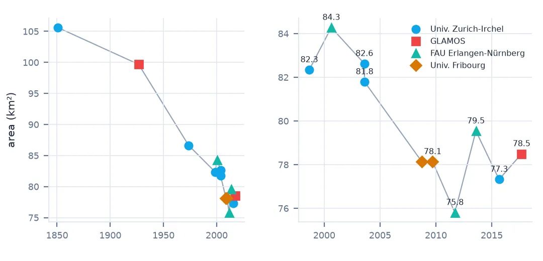
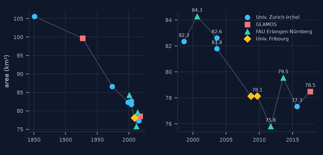
Glacier inventories — the Randolph Glacier Inventory, the GLIMS database, national inventories — give every glacier an outline, an identifier and an area. Download several records of one glacier and plot their areas against time, and the line does not fall smoothly: records two years apart differ by more than the glacier could have changed, a later outline is larger than an earlier one, and two outlines with the same date disagree. None of these are errors in the usual sense. They are what happens when "the glacier" is a decision made by whoever drew the line.

This page reads every GLIMS record of the Great Aletsch Glacier in Switzerland, from a reconstruction of 1850 to a GLAMOS outline of 2017, and measures where and why they disagree.

Quick answer

Fetch the outlines from the GLIMS web feature service, keep the main glacier boundary of each record, compute areas in a metric CRS, and look at who drew each one:

g = gpd.read_file(GLIMS_WFS)
a = g[(g.glac_id == "G008032E46504N") & (g.line_type == "glac_bound")].to_crs(2056)
a = a[a.area > 1e6].sort_values("src_date")
a["km2"] = (a.area / 1e6).round(2)
print(a[["src_date", "chief_affl", "km2"]].assign(src_date=a.src_date.dt.date).to_string(index=False))

  src_date                              chief_affl    km2
1850-09-01             University of Zurich-Irchel 105.62
1926-09-01 GLAMOS (Glacier Monitoring Switzerland)  99.68
1973-09-01             University of Zurich-Irchel  86.63
1998-08-31             University of Zurich-Irchel  82.34
2000-08-20    Friedrich-Alexander University (FAU)  84.28
2003-08-06             University of Zurich-Irchel  82.63
2003-08-13             University of Zurich-Irchel  81.79
2008-09-30                  University of Fribourg  78.13
2009-09-15                  University of Fribourg  78.13
2011-09-13    Friedrich-Alexander University (FAU)  75.80
2013-08-01    Friedrich-Alexander University (FAU)  79.54
2015-08-29             University of Zurich-Irchel  77.32
2017-09-01 GLAMOS (Glacier Monitoring Switzerland)  78.49

What a record is, and why outlines differ

1. Know what a record is

A GLIMS record is one analysis: an analyst, a source image or map with a date, and a set of lines — the glacier boundary, debris-covered parts, rock outcrops inside. The glacier keeps one identifier across records, so the same glac_id collects outlines from different people, methods and decades:

print(g.line_type.value_counts().to_dict())
print(a.groupby("chief_affl").size().to_dict())

{'glac_bound': 1362, 'debris_cov': 342}
{'Friedrich-Alexander University (FAU)': 3, 'GLAMOS (Glacier Monitoring Switzerland)': 2, 'University of Fribourg': 2, 'University of Zurich-Irchel': 6}

2. Same date, different outline

Two University of Zurich records are dated a week apart in August 2003:

d1, d2 = (make_valid(a[a.src_date.dt.strftime("%Y-%m-%d") == d].geometry.iloc[0]) for d in ("2003-08-06", "2003-08-13"))
print(f"areas {d1.area / 1e6:.2f} and {d2.area / 1e6:.2f} km²; drawn differently over {d1.symmetric_difference(d2).area / 1e6:.2f} km²")

areas 82.63 and 81.79 km²; drawn differently over 1.19 km²

A glacier does not lose 0.8 km² in a week. The difference is in the drawing: which rock outcrops are cut out, where a steep upper edge is placed. More than a square kilometre of the two outlines disagree.

3. Later is not always smaller

FAU's 2013 record is larger than its own 2011 record:

for y1, y2 in ((1998, 2000), (2011, 2013), (2015, 2017)):
    A, B = (make_valid(a[a.src_date.dt.year == y].geometry.iloc[-1]) for y in (y1, y2))
    print(f"{y1} -> {y2}: area {(B.area - A.area) / 1e6:+.2f} km²; added {B.difference(A).area / 1e6:.2f}, removed {A.difference(B).area / 1e6:.2f}")

1998 -> 2000: area +1.94 km²; added 3.60, removed 1.66
2011 -> 2013: area +3.74 km²; added 5.10, removed 1.36
2015 -> 2017: area +1.17 km²; added 2.68, removed 1.51

Every pair "added" ice somewhere as well as removing it. Added ice on a retreating glacier is almost always a boundary drawn more generously — a snow-covered slope included, a divide moved — not growth.

4. Glaciers split

The Mittelaletsch flowed into the Great Aletsch in 1850 and was part of it in the 1850 reconstruction. By 1973 it was inventoried as a glacier of its own, and its own record has since broken into fragments:

mittel = g[(g.glac_id == "G008010E46463N") & (g.line_type == "glac_bound")].to_crs(2056).sort_values("src_date")
print(mittel.assign(km2=(mittel.area / 1e6).round(2), date=mittel.src_date.dt.date)[["date", "km2"]].to_string(index=False))

      date  km2
1973-09-01 8.31
1998-08-31 7.49
2003-08-06 7.43
2003-08-13 7.50
2008-09-30 5.39
2009-09-15 1.00
2011-09-13 0.91
2015-08-29 0.03

When a tributary separates, the main glacier's area drops by the tributary's whole area at once — about 8 km² here, a tenth of the glacier — without any ice melting. A time series of one identifier's area mixes that step in with the real retreat.

5. Use records carefully

For change over time, use records from one inventory with one set of rules (GLAMOS for Switzerland, RGI for global work), compare outlines rather than just areas, and treat a difference between analysts as a measure of uncertainty, not of change.

Spread between analysts as uncertainty

The data used on this page

GLIMS Glacier Database (Global Land Ice Measurements from Space, NSIDC), web feature service layer GLIMS_Glacier_Outlines, records for Grosser Aletschgletscher (G008032E46504N) and Mittelaletschgletscher (G008010E46463N). Submissions by the University of Zurich, GLAMOS (Glacier Monitoring Switzerland), Friedrich-Alexander-Universität Erlangen-Nürnberg and the University of Fribourg.

from pathlib import Path

import geopandas as gpd
import requests
from shapely import make_valid

Path("data").mkdir(exist_ok=True)
URL = ("https://www.glims.org/geoserver/GLIMS/ows?service=WFS&version=1.0.0&request=GetFeature"
       "&typeName=GLIMS:GLIMS_Glacier_Outlines&outputFormat=application/json&bbox=7.95,46.40,8.15,46.56")
GLIMS_WFS = "data/glims_aletsch.json"
if not Path(GLIMS_WFS).exists():
    Path(GLIMS_WFS).write_bytes(requests.get(URL, timeout=300).content)
print(Path(GLIMS_WFS).stat().st_size // 1_000_000, "MB of GeoJSON")

11 MB of GeoJSON

Example 1: the spread between analysts as an uncertainty

Records within three years of each other by different analysts bound how well "the area" is known at one time:

recent = a[a.src_date.dt.year >= 1998].assign(year=a.src_date.dt.year)
for centre in (2000, 2010, 2015):
    near = recent[(recent.year - centre).abs() <= 3]
    print(f"{centre} ± 3 years: {len(near)} records, {near.km2.min():.1f}-{near.km2.max():.1f} km² "
          f"(spread {near.km2.max() - near.km2.min():.1f})")

2000 ± 3 years: 4 records, 81.8-84.3 km² (spread 2.5)
2010 ± 3 years: 4 records, 75.8-79.5 km² (spread 3.7)
2015 ± 3 years: 3 records, 77.3-79.5 km² (spread 2.2)

A spread of several square kilometres around 2010 is larger than the glacier's real change over five years. Any trend computed across analysts has to be larger than that to mean anything.

Example 2: debris is part of the glacier

GLIMS marks debris-covered ice separately. GLAMOS's 2017 record has dozens of debris polygons:

debris = g[(g.glac_id == "G008032E46504N") & (g.line_type == "debris_cov")].to_crs(2056)
print(f"{len(debris)} debris polygons, {debris.area.sum() / 1e6:.2f} km², dated {sorted(set(debris.src_date.dt.year))}")

76 debris polygons, 4.71 km², dated [2017]

Debris-covered ice is glacier, but it is the hardest part to map from imagery because it looks like the moraine beside it. Inventories that omit it understate area, and those that include it do so with less certainty.

An inventory is a set of decisions

A glacier inventory is a set of decisions written as geometry. Where does one glacier end and its neighbour begin? Is a steep rock face with a few ice patches inside or out? Is debris-covered ice included? Is a tributary that touches the main glacier only at its snout part of it? Each inventory answers these with rules, and different inventories — or different analysts within one — answer them differently.

The result is that a glacier's area carries two kinds of change: real change in the ice, and change in the rules. On the Great Aletsch, the real retreat of the tongue is unmistakable in every record — a steady climb of the terminus up its valley. The area series, meanwhile, includes a step of about 8 km² when the Mittelaletsch was split off, week-apart records differing by 0.8 km², and two-year-apart records from the same group differing by almost 4 km² in the wrong direction.

The remedy is not to distrust inventories but to read them as what they are: careful, documented interpretations. Use one consistent inventory for change, look at outlines and not just areas, and use the disagreement between analysts as an estimate of uncertainty.

Many analysts, tributaries and fragments

• One identifier, many analysts. Group GLIMS records by chief_affl before computing change.
• Tributaries separate; a step in area may be a split, not melt.
• Records include fragments; keep the main glac_bound polygon or sum deliberately.
• Debris-covered ice is stored as separate debris_cov lines.
• Invalid geometries occur; run make_valid before overlays.
• RGI is a snapshot around 2000 for each glacier; use GLIMS or national inventories for time series.

Internal links

• How to compute glacier hypsometry from a DEM — what these outlines say about elevation
• How to measure glacier retreat — terminus change, robust to boundary choices
• How accurate is a historical map? — the 1850 outline is a reconstruction
• How to measure change from an old map — definitions at two dates
• Snow cover and NDSI explained — mapping ice and snow from imagery

FAQ

Why do glacier areas differ between inventories?

Inventories draw boundaries between glaciers, around rock outcrops and over debris by different rules, and their source images and dates differ. On the Great Aletsch, records a week apart differ by 0.8 km².

What is the GLIMS database?

The Global Land Ice Measurements from Space glacier database, hosted by NSIDC, collecting glacier outlines from many analysts and dates, each tagged with the analyst and source date.

Can a glacier's inventory area increase while it retreats?

Yes — a boundary drawn more generously in a later record can add more area than the glacier lost. FAU's 2013 Great Aletsch outline is 3.7 km² larger than its 2011 one.

How do I compare glacier areas over time?

Use records from one inventory with consistent rules, compare the outlines themselves, and treat differences between analysts as uncertainty rather than change.