Marine Heatwaves Explained

Problem statement

"Marine heatwave" entered common use around 2016, after the Pacific "Blob" and the bleaching of the Great Barrier Reef, and with it came a need for a definition precise enough to count. A fixed temperature threshold does not work across oceans whose normal temperatures differ by 30 °C, and a fixed anomaly does not work across seasons whose variability differs. The definition now in wide use, from Hobday and colleagues, is relative to the local seasonal cycle, and it has consequences that are easy to miss: a heatwave can be colder than an ordinary summer day, and a warming ocean will eventually be in "permanent heatwave" against a fixed baseline.

This page explains the definition, its metrics and categories, and its baseline choices, using 42 years of daily OISST for a box off the west of Ireland and the record event of June 2023.

Quick answer

Detect events against the seasonally varying 90th percentile of 1991–2020, then describe each by its duration and intensity:

e = EV.loc[EV.days.idxmax()]
x = (T - CLIM)[e.start:e.end]
print(f"longest event: {e.start:%d %b %Y} to {e.end:%d %b %Y}, {e.days} days")
print(f"intensity: mean {x.mean():.2f} °C, maximum {x.max():.2f} °C on {x.idxmax():%d %b}, cumulative {x.sum():.0f} °C days")
print(f"peak relative to the local threshold distance: {((T - CLIM) / (THRESH - CLIM))[e.start:e.end].max():.2f}x")

longest event: 31 Jul 1995 to 19 Sep 1995, 51 days
intensity: mean 1.62 °C, maximum 2.45 °C on 17 Aug, cumulative 83 °C days
peak relative to the local threshold distance: 2.60x

The longest event in 42 years ran from 31 July to 19 September 1995, 51 days. On average it was 1.62 °C above the seasonal normal and at most 2.45 °C, an accumulated 83 °C-days, and its peak was 2.6 times the local distance between threshold and mean: a strong event, long rather than intense. The June 2023 event was shorter but more intense.

Relative to season, categories, the baseline and the trend

1. Relative to the season

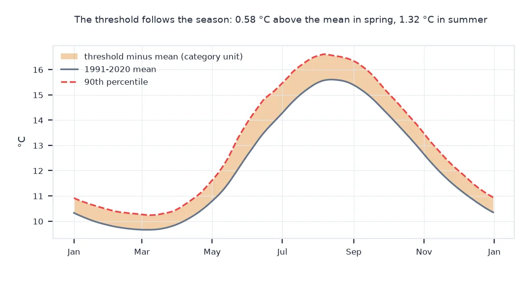
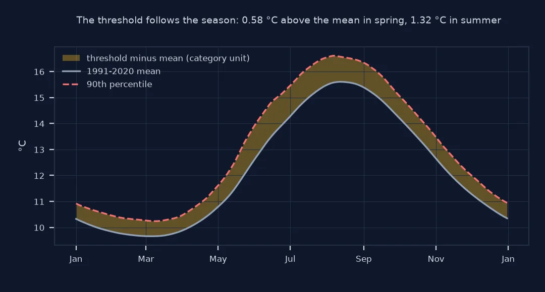
The threshold follows the seasonal cycle. Compare a winter heatwave day with an ordinary summer day:

winter = EV[EV.start.dt.month.isin([12, 1, 2])]
if len(winter):
    w = winter.iloc[-1]; d = (T - THRESH)[w.start:w.end].idxmax()
    print(f"winter event {w.start:%d %b %Y}: on {d:%d %b} the sea was {T[d]:.2f} °C, {T[d] - CLIM[d]:+.2f} °C above normal")
print(f"an ordinary August day: climatology {CLIM[CLIM.index.month == 8].mean():.2f} °C, threshold {THRESH[THRESH.index.month == 8].mean():.2f} °C")
print(f"threshold above climatology: {float((THRESH - CLIM).min()):.2f} to {float((THRESH - CLIM).max()):.2f} °C through the year")

winter event 25 Feb 2023: on 28 Feb the sea was 10.36 °C, +0.69 °C above normal
an ordinary August day: climatology 15.55 °C, threshold 16.52 °C
threshold above climatology: 0.58 to 1.32 °C through the year

On 28 February 2023 the sea was 10.36 °C, 0.69 °C above normal and inside a heatwave, while an ordinary August day has a normal of 15.55 °C and a threshold of 16.52 °C. The winter heatwave was more than 5 °C colder than a normal summer day. The threshold sits 0.58 to 1.32 °C above the mean, depending on the season's variability.

2. Categories

Categories scale each event's peak by the local distance between threshold and climatology: I moderate, II strong, III severe, IV extreme. Show how intensity in degrees and category relate:

peaks = [((T - CLIM) / (THRESH - CLIM))[s:e].max() for s, e in zip(EV.start, EV.end)]
deg = [(T - CLIM)[s:e].max() for s, e in zip(EV.start, EV.end)]
cat = pd.cut(peaks, [1, 2, 3, 4, 99], right=False, labels=["I moderate", "II strong", "III severe", "IV extreme"])
t = pd.DataFrame({"category": cat, "peak_degC": deg}).groupby("category", observed=False).peak_degC.agg(["size", "min", "max"]).round(2)
print(t.to_string())

            size   min   max
category                    
I moderate    68  0.69  2.21
II strong     16  1.22  3.15
III severe     4  2.90  3.74
IV extreme     0   NaN   NaN

Categories overlap in degrees: a moderate event can peak 2.21 °C above normal in summer and a strong one 1.22 °C in winter, because each is scaled by its season's variability. The four severe events peaked 2.90 to 3.74 °C above normal; none reached extreme.

3. The baseline decides the trend

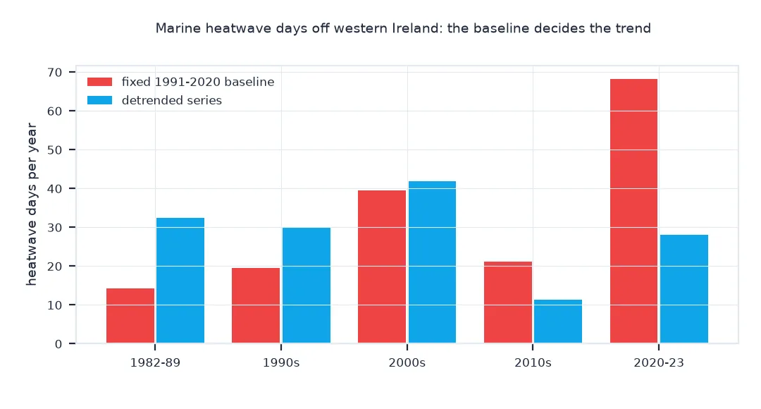
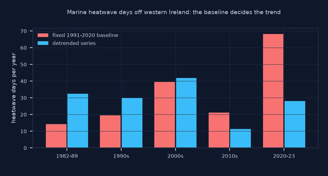
Against a fixed baseline, warming adds heatwave days. Detrend the series first, and the count measures departures from the moving normal instead:

trend = np.polyfit(np.arange(len(T)), T.values, 1)
detr = T - np.polyval(trend, np.arange(len(T))) + np.polyval(trend, np.arange(len(T))).mean()
c2, t2 = climatology(detr, "1991-01-01", "2020-12-31")
ev2 = events(detr > t2)
years = pd.Series(sorted(set(T.index.year)))
per_decade = years.groupby(years // 10 * 10).size()                                # 1980s and 2020s are partial
for label, ev in (("fixed 1991-2020 baseline", EV), ("detrended", ev2)):
    d = ev.set_index("start").days.groupby(lambda i: (i.year // 10) * 10).sum() / per_decade
    print(f"{label:>25}: heatwave days per year by decade: {d.round(0).astype(int).to_dict()}")
print(f"warming trend in the box: {trend[0] * 3652.5:+.2f} °C per decade")

 fixed 1991-2020 baseline: heatwave days per year by decade: {1980: 14, 1990: 19, 2000: 39, 2010: 21, 2020: 68}
                detrended: heatwave days per year by decade: {1980: 32, 1990: 30, 2000: 42, 2010: 11, 2020: 28}
warming trend in the box: +0.21 °C per decade

The box warmed at 0.21 °C per decade over 1982–2023. Against the fixed baseline, heatwave days rise from 14 a year in the 1980s to 68 a year in 2020–2023. With the trend removed, the 1980s and 1990s gain heatwave days, 32 and 30 a year, and the 2010s and 2020–2023 lose them, 11 and 28: much of the rise in the fixed-baseline count is the trend, though the 2020s still stand out in the detrended one.

A fixed threshold instead

The data used on this page

Daily NOAA OISST from 1982 to 2023 for 52°N to 54°N and 12°W to 10°W, averaged with cosine-of-latitude weights, with every day present, as in the marine heatwave detection guide. The definition and categories follow Hobday et al. (2016) and Hobday et al. (2018), Oceanography 31(2).

import io
import time
from pathlib import Path

import numpy as np
import pandas as pd
import requests
import xarray as xr

Path("data").mkdir(exist_ok=True)
CW = "https://coastwatch.pfeg.noaa.gov/erddap/griddap"
ARCHIVE = "https://www.ncei.noaa.gov/data/sea-surface-temperature-optimum-interpolation/v2.1/access/avhrr"
def _get(url):
    for attempt in range(5):                                            # a busy ERDDAP answers 500 or 503
        r = requests.get(url, timeout=900)
        if r.status_code < 500:
            break
        time.sleep(30 * (attempt + 1))
    r.raise_for_status()
    return r
def _lon180(da):
    return da.assign_coords(longitude=(da.longitude + 180) % 360 - 180).sortby("longitude")
def oisst(start, end, path, var="sst", lat=(52, 54), lon=(-12, -10), step=1):
    """Daily OISST v2.1 for a box and dates, saved to path, longitudes -180 to 180. CoastWatch's ERDDAP
    aggregation (version 2 before 2016, the same analysis as v2.1 for those years), with every day it
    lacks taken from NCEI's daily archive: the aggregations skip days, and a skipped day is silent."""
    path = Path(path)
    if not path.exists():
        days = pd.date_range(start, end)
        ds = "ncdcOisst2Agg" if days[-1].year <= 2015 else "ncdcOisst21Agg"
        a, b = lon[0] % 360, lon[1] % 360
        got = []
        for lo in [(a, b)] if a <= b else [(a, 359.875), (0.125, b)]:          # across 0°, two requests
            q = (f"{var}[({start}T12:00:00Z):1:({end}T12:00:00Z)][(0.0)]"
                 f"[({lat[0]}):{step}:({lat[1]})][({lo[0]}):{step}:({lo[1]})]")
            got.append(xr.open_dataset(io.BytesIO(_get(f"{CW}/{ds}.nc?{q}").content))[var].load())
        da = _lon180(xr.concat(got, "longitude").squeeze("zlev", drop=True))
        da = da.sel(time=slice(start, f"{end}T23:59"))                       # a missing end day snaps past it
        for day in days.difference(pd.DatetimeIndex(da.time.values).normalize()):
            url = f"{ARCHIVE}/{day:%Y%m}/oisst-avhrr-v02r01.{day:%Y%m%d}.nc"
            d = xr.open_dataset(io.BytesIO(_get(url).content))[var].squeeze("zlev", drop=True)
            d = _lon180(d.rename(lat="latitude", lon="longitude"))
            d = d.sel(latitude=da.latitude, longitude=da.longitude, method="nearest")
            da = xr.concat([da, d.assign_coords(latitude=da.latitude, longitude=da.longitude).load()], "time")
        da.sortby("time").to_dataset(name=var).to_netcdf(path)
    return xr.open_dataset(path)[var]
def oisst_year(year, var="sst", lat=(52, 54), lon=(-12, -10), tag="ireland_west"):
    return oisst(f"{year}-01-01", f"{year}-12-31", f"data/oisst_{tag}_{var}_{year}.nc", var, lat, lon)
da = xr.concat([oisst_year(y) for y in range(1982, 2024)], "time")
T = da.weighted(np.cos(np.deg2rad(da.latitude))).mean(["latitude", "longitude"]).to_series()
T.index = T.index.normalize()
def climatology(t, start, end, window=5, smooth=31):
    d = t.index.dayofyear - ((t.index.is_leap_year) & (t.index.dayofyear > 59)).astype(int)
    d = np.where((t.index.month == 2) & (t.index.day == 29), 59, d)
    base = pd.Series(t.values, index=d)[(t.index >= start) & (t.index <= end)]
    m, p = {}, {}
    for k in range(1, 366):
        v = base[base.index.isin([(k + o - 1) % 365 + 1 for o in range(-window, window + 1)])]
        m[k], p[k] = v.mean(), v.quantile(0.9)
    sm = lambda s: pd.concat([s.iloc[-smooth:], s, s.iloc[:smooth]]).rolling(smooth, center=True).mean().iloc[smooth:-smooth]
    m, p = sm(pd.Series(m)), sm(pd.Series(p))
    return pd.Series(m.loc[d].values, index=t.index), pd.Series(p.loc[d].values, index=t.index)
def events(hot, min_days=5, max_gap=2):
    r = (hot != hot.shift()).cumsum()
    runs = [(g.index[0], g.index[-1]) for _, g in hot[hot].groupby(r[hot]) if len(g) >= min_days]
    joined = []
    for s, e in runs:
        if joined and (s - joined[-1][1]).days - 1 <= max_gap:
            joined[-1] = (joined[-1][0], e)
        else:
            joined.append((s, e))
    return pd.DataFrame({"start": [s for s, _ in joined], "end": [e for _, e in joined], "days": [(e - s).days + 1 for s, e in joined]})
CLIM, THRESH = climatology(T, "1991-01-01", "2020-12-31")
EV = events(T > THRESH)
print(f"{len(T):,} days; {len(EV)} events against the fixed 1991-2020 baseline")

15,340 days; 88 events against the fixed 1991-2020 baseline

The series has 15,340 days and 88 events against the fixed 1991–2020 baseline.

Example 1: a fixed threshold instead

A simpler rule, any five days at least 2 °C above the climatology, treats all seasons alike. Compare what it finds:

fixed = events((T - CLIM) >= 2.0)
print(f"percentile definition: {len(EV)} events, {EV.days.sum():,} days; fixed +2 °C: {len(fixed)} events, {fixed.days.sum():,} days")
print(f"months of fixed-threshold events: {fixed.start.dt.month.value_counts().sort_index().to_dict()}")

percentile definition: 88 events, 1,186 days; fixed +2 °C: 11 events, 113 days
months of fixed-threshold events: {5: 2, 6: 4, 7: 3, 8: 2}

A fixed rule of 2 °C above normal finds 11 events and 113 days, all between May and August, against 88 events and 1,186 days with the percentile definition. Because summer temperatures vary most, a fixed anomaly reaches the threshold only in summer and misses every winter and spring heatwave.

The Hobday definition

Hobday and colleagues defined a marine heatwave in 2016 as a discrete, prolonged, anomalously warm water event: at least five days above the 90th percentile of a 30-year climatology for that time of year, with gaps of up to two days bridged. Every part of that sentence is a choice. Discrete and prolonged rule out a single warm day. Anomalous relative to the time of year means a heatwave can occur in winter. The 90th percentile, rather than a fixed anomaly, scales the threshold to local variability, so places with naturally steady temperatures need smaller departures. Events are then described by duration, mean and maximum intensity, cumulative intensity in degree days, and rates of onset and decline.

The categories, added in 2018, express peak intensity as a multiple of the gap between the threshold and the mean, an analogy to hurricane categories that makes events comparable across regions. The baseline is the decision with the largest effect over long periods. A fixed historical baseline treats warming as part of the signal, so heatwave days rise with the trend and eventually become the norm; a detrended or moving baseline treats warming as the new normal and counts only departures from it. Both are defensible; they answer whether the ocean is warmer than it was, and whether it is unusually warm for now.

Cold spells, depth and box size

• Cold spells: the same method with the 10th percentile and temperatures below it defines marine cold spells.
• Depth: the definition uses surface temperature; heatwaves below the surface, which matter for many organisms, need subsurface data such as Argo profiles.
• Box size: averaging a box before detection smooths the series and reduces the number of events relative to running the method cell by cell.
• Baseline length: shorter records give noisier percentiles; OISST supports 1991–2020, while 1983–2012 was the original choice when the definition was published.

Internal links

• How to detect marine heatwaves in Python — the method step by step
• How to map marine heatwave days in Python — the method on a grid
• Degree heating weeks explained — the measure built for coral stress

FAQ

What is a marine heatwave?

A period of at least five days when sea surface temperature is above the seasonally varying 90th percentile of a 30-year climatology for that place and time of year.

What are the categories of marine heatwaves?

Moderate, strong, severe and extreme, when the peak reaches one, two, three or four times the local difference between the 90th percentile and the mean.

Can a marine heatwave happen in winter?

Yes: the threshold follows the season, so unusually warm winter water counts even though it is colder than a typical summer.

Will warming make marine heatwaves permanent?

Against a fixed historical baseline, yes, eventually; against a moving or detrended baseline, heatwaves remain departures from the recent normal.