Fixing Global SST Means That Ignore Cell Area

Problem statement

A global or basin-wide mean sea surface temperature computed with .mean() over latitude and longitude comes out several degrees too cold, and its trend is off. Every cell of a latitude-longitude grid gets the same weight, but cells near the poles cover a fraction of the area of cells near the equator, so the cold high latitudes are counted far more than their share of the ocean. The error is invisible in the code and plausible in the result.

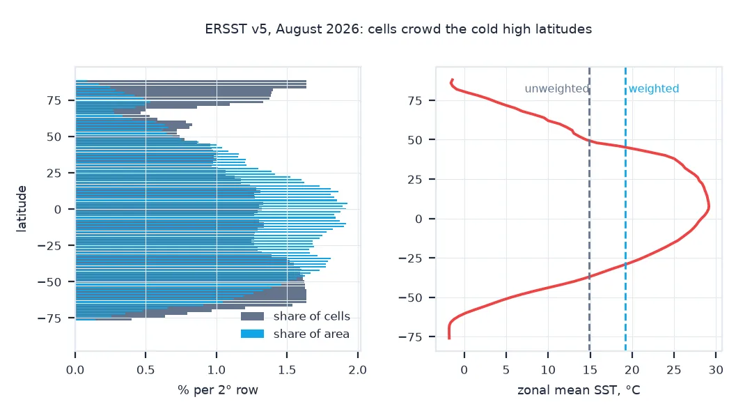
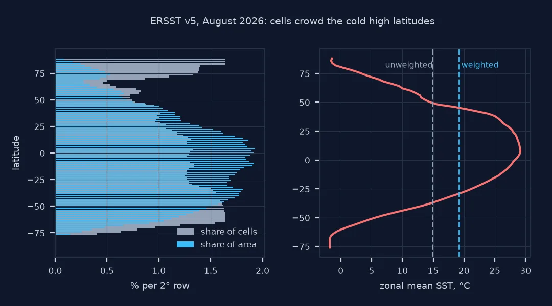
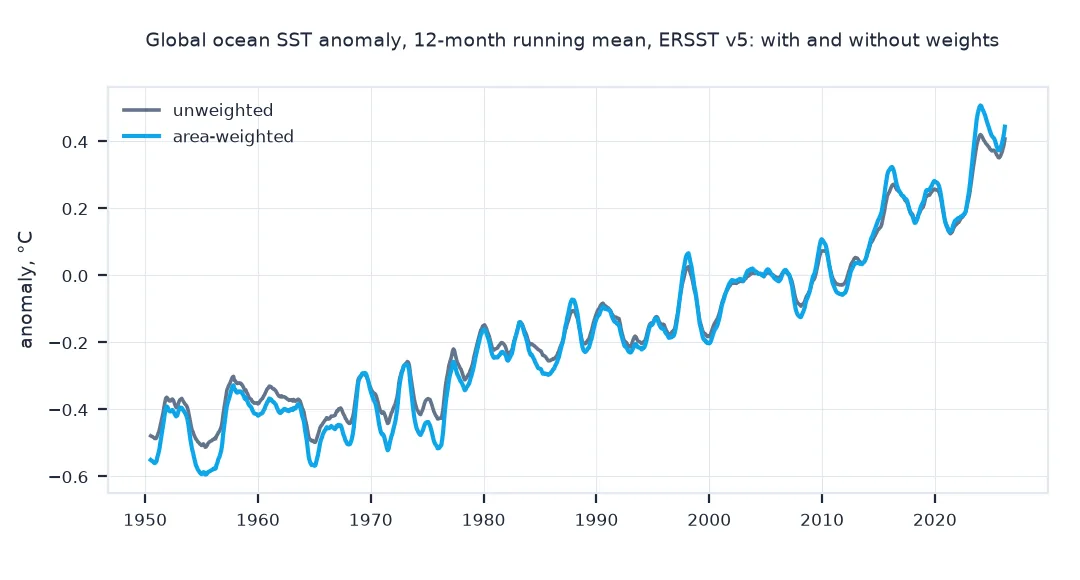
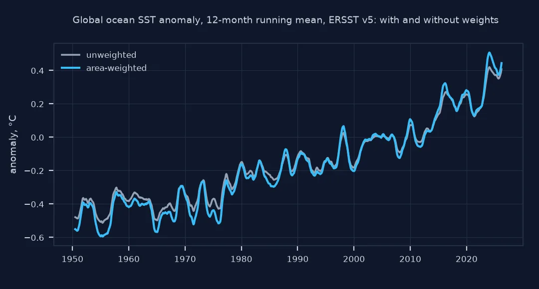
This page computes the global mean of ERSST v5 with and without area weights, shows where the cells and the area are, measures the error in the mean, the anomalies and the trend, and checks the cosine weight against exact cell areas.

Quick answer

Pass cosine-of-latitude weights to xarray's weighted before averaging:

last = SST.isel(time=-1)
naive = float(last.mean())
w = np.cos(np.deg2rad(last.latitude))
right = float(last.weighted(w).mean())
print(f"{pd.Timestamp(last.time.values):%B %Y}: unweighted mean {naive:.2f} °C, area-weighted {right:.2f} °C, error {naive - right:+.2f} °C")

August 2026: unweighted mean 14.91 °C, area-weighted 19.16 °C, error -4.25 °C

Without weights the global ocean averages 14.91 °C in August 2026; with them, 19.16 °C. The unweighted mean is 4.25 °C too cold.

Cells against area, effects on anomalies and trends, exact areas

1. Cells against area

Count the ocean cells and their share of the ocean area in latitude bands:

ocean = last.notnull()
band = pd.cut(np.abs(ocean.latitude.values), [0, 30, 60, 90], labels=["0-30°", "30-60°", "60-90°"])
c = ocean.sum("longitude").to_series().groupby(band).sum()
a = (ocean * w).sum("longitude").to_series().groupby(band).sum()
print(pd.DataFrame({"share of cells": (c / c.sum()).map("{:.0%}".format), "share of area": (a / a.sum()).map("{:.0%}".format)}).to_string())

       share of cells share of area
0-30°             38%           52%
30-60°            37%           38%
60-90°            25%           10%

Cells poleward of 60° are a quarter of all ocean cells but a tenth of the ocean area; the tropics are 38% of cells and 52% of the area. An unweighted mean gives the polar seas two and a half times their share.

2. What it does to anomalies and trends

Compute monthly global means both ways for the whole record, turn them into anomalies against 1991–2020, and compare the trend:

def series(weighted):
    s = (SST.weighted(np.cos(np.deg2rad(SST.latitude))) if weighted else SST).mean(["latitude", "longitude"]).to_series()
    c = s["1991":"2020"].groupby(s["1991":"2020"].index.month).mean()
    return s - s.index.month.map(c).values
u, wtd = series(False), series(True)
x = np.arange(len(u["1982":"2025"]))
print(f"trend 1982-2025: unweighted {np.polyfit(x, u['1982':'2025'], 1)[0] * 120:+.3f}, weighted {np.polyfit(x, wtd['1982':'2025'], 1)[0] * 120:+.3f} °C per decade")
print(f"largest monthly anomaly difference: {float((u - wtd).abs().max()):.2f} °C")

trend 1982-2025: unweighted +0.125, weighted +0.136 °C per decade
largest monthly anomaly difference: 0.12 °C

The anomaly series differ by up to 0.12 °C in a month, and the trend since 1982 is 0.125 °C per decade unweighted against 0.136 weighted, because the over-weighted high-latitude cells changed at different rates from the tropics.

3. Cosine weights against exact cell areas

For a regular grid, a cell's area is proportional to the difference of the sines of its edge latitudes, and the cosine of its centre latitude is almost exactly proportional to that:

half = 1.0                                                                           # ERSST cells are 2° tall
exact = np.sin(np.deg2rad(last.latitude + half).clip(-90, 90)) - np.sin(np.deg2rad(last.latitude - half).clip(-90, 90))
exact = xr.DataArray(np.abs(exact.values), coords={"latitude": last.latitude})
print(f"mean with cos weights {right:.4f} °C, with exact areas {float(last.weighted(exact).mean()):.4f} °C")
r = (exact / w).values
print(f"exact / cos ratio across latitudes: {r.min():.5f} to {r.max():.5f}")

mean with cos weights 19.1599 °C, with exact areas 19.1599 °C
exact / cos ratio across latitudes: 0.03490 to 0.03490

Exact cell areas and cosine weights give the same mean to four decimals: on a regular grid the ratio between them is the same constant at every latitude, so the weights are proportional.

A regional mean has the same problem

The data used on this page

Monthly NOAA ERSST v5 on its 2° grid from January 1950 to August 2026, from NOAA CoastWatch's ERDDAP.

from pathlib import Path

import numpy as np
import pandas as pd
import requests
import xarray as xr

Path("data").mkdir(exist_ok=True)
p = Path("data/ersst_global_1950_202608.nc")
if not p.exists():
    q = "sst[(1950-01-01):1:(2026-08-01)][(0.0)][(-88):1:(88)][(-180):1:(178)]"
    p.write_bytes(requests.get(f"https://coastwatch.pfeg.noaa.gov/erddap/griddap/nceiErsstv5_LonPM180.nc?{q}", timeout=900).content)
SST = xr.open_dataset(p).sst.squeeze(drop=True)
print(f"{SST.sizes['time']} months; latitudes {float(SST.latitude.min())} to {float(SST.latitude.max())} every {float(SST.latitude[1] - SST.latitude[0])}°")

920 months; latitudes -88.0 to 88.0 every 2.0°

The grid has 89 rows from 88°S to 88°N, 2° apart.

Example 1: a regional mean has the same problem

The error is not only global. Compare the two means for the North Atlantic from the equator to 70°N:

na = last.sel(latitude=slice(0, 70), longitude=slice(-80, 0))
print(f"North Atlantic, {pd.Timestamp(last.time.values):%b %Y}: unweighted {float(na.mean()):.2f} °C, weighted {float(na.weighted(np.cos(np.deg2rad(na.latitude))).mean()):.2f} °C")

North Atlantic, Aug 2026: unweighted 21.48 °C, weighted 23.47 °C

For the North Atlantic between the equator and 70°N the unweighted mean is 2 °C too cold, 21.48 against 23.47 °C.

Equal angles, unequal areas

On a latitude-longitude grid every cell spans the same angles, but a degree of longitude covers 111 km at the equator and nothing at the poles. The area of a cell is proportional to the cosine of its latitude, so a cell at 60° is half the size of one at the equator and a cell at 80° about a sixth. An unweighted mean treats them as equal, which in the ocean gives the cold Southern Ocean and Arctic seas much more influence than their area, and pulls the mean down by several degrees.

Trends are affected less than levels, because the bias in level is roughly constant, but not zero: high latitudes warm at different rates from the tropics, so over-weighting them changes the slope. The fix is a weight per cell: the cosine of the centre latitude for a regular grid, which matches exact areas to within a fraction of a percent, or the actual cell area for any other grid. Land and ice masks need no special handling in xarray's weighted, which ignores missing values and normalises by the weights of the cells that remain.

Missing data, anomalies and curvilinear grids

• Weights and missing data: weighted(w).mean() normalises by the sum of weights over non-missing cells; a manual (x * w).sum() / w.sum() over all cells is wrong where cells are missing.
• Means of anomalies: averaging anomaly fields needs the same weights as averaging temperatures.
• Projected or curvilinear grids: ocean models on tripolar or rotated grids provide a cell-area variable (areacello in CMIP output); use it.
• Polar cells: cells centred at ±88° are tiny; the clip in the exact-area formula keeps their edges at ±90°.

Internal links

• How to compute the global mean sea surface temperature in Python — the weighted series in detail
• How to take an area-weighted mean over a latitude–longitude grid — the same issue for any variable
• How to map sea surface temperature trends in Python — trends per cell and their global mean

FAQ

Why is my global mean sea surface temperature too cold?

It was probably averaged without area weights, so small high-latitude cells count as much as large tropical ones; weight by the cosine of latitude.

How do I compute an area-weighted mean in xarray?

da.weighted(np.cos(np.deg2rad(da.latitude))).mean(["latitude", "longitude"]).

Is cosine of latitude the exact area weight?

For a regular latitude-longitude grid it is proportional to the exact cell area to within a fraction of a percent; use true cell areas on other grids.

Do I need weights for anomalies too?

Yes; any spatial mean over a latitude-longitude grid needs them, whatever the variable.