How to Compute an El Niño Index from Sea Surface Temperature in Python

Problem statement

El Niño and La Niña are diagnosed from the temperature of one patch of the equatorial Pacific, the Niño 3.4 region from 5°S to 5°N and 170°W to 120°W. NOAA's Climate Prediction Center turns monthly ERSST temperatures there into the Oceanic Niño Index (ONI): a three-month running mean of anomalies, with El Niño declared when it stays at or above +0.5 °C for five overlapping seasons. Computing it yourself means averaging the right cells, choosing a base period, and smoothing in the right order, and checking the result against CPC's published values shows whether those choices were right.

This page downloads ERSST v5 for the Niño 3.4 box since 1950, computes the region mean, anomalies and the three-month index, compares it with CPC's ONI, and finds the El Niño and La Niña episodes, including the one under way in 2026.

Quick answer

Average the box with area weights, subtract each calendar month's base-period mean, and take a centred three-month mean:

n34 = box.weighted(np.cos(np.deg2rad(box.latitude))).mean(["latitude", "longitude"]).to_series()
n34.index = n34.index.to_period("M").to_timestamp()                       # ERDDAP stamps ERSST on the 1st to 2007, the 15th after
clim = n34["1991":"2020"].groupby(n34["1991":"2020"].index.month).mean()
anom = n34 - n34.index.month.map(clim).values
oni = anom.rolling(3, center=True).mean()
print(f"Niño 3.4 from {n34.index[0]:%b %Y} to {n34.index[-1]:%b %Y}; latest three-month index ({oni.dropna().index[-1]:%b %Y} centre): {oni.dropna().iloc[-1]:+.2f} °C")
print(f"CPC ONI for the same season: {CPC.iloc[-1]:+.2f} °C")

Niño 3.4 from Jan 1950 to Aug 2026; latest three-month index (Jul 2026 centre): +2.00 °C
CPC ONI for the same season: +1.80 °C

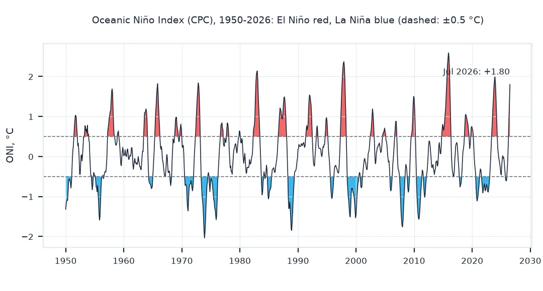
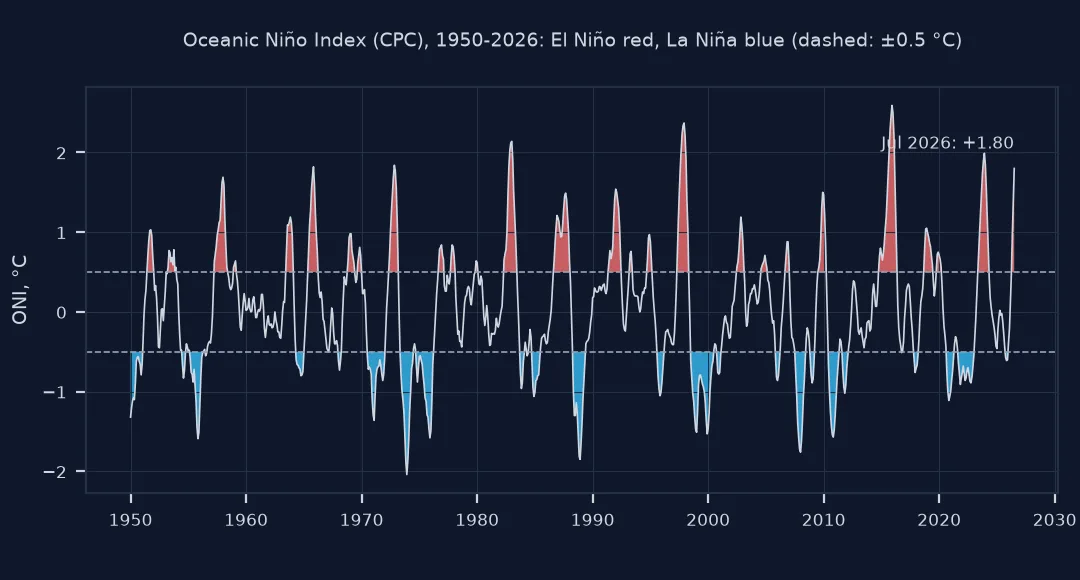
The latest complete three-month window is June to August 2026, centred on July. Against a fixed 1991–2020 base, Niño 3.4 is 2.00 °C above normal; CPC's ONI for the same season is +1.80 °C. Both put the Pacific firmly in El Niño conditions; the gap between them is the base period, as Example 1 shows.

Which cells are in the box, against CPC, episodes

1. Which cells are in the box

ERSST's 2° cells are centred on even degrees, so the box's edges at 5°S and 5°N fall between cell centres. Keep the cells whose centres lie inside it:

print(f"latitudes kept: {box.latitude.values.tolist()}; longitudes {float(box.longitude.min()):.0f} to {float(box.longitude.max()):.0f} ({box.sizes['longitude']} columns)")
print(f"months: {n34.size}; Niño 3.4 range {n34.min():.2f} to {n34.max():.2f} °C; mean seasonal cycle from {clim.min():.2f} °C ({clim.idxmin()}) to {clim.max():.2f} °C ({clim.idxmax()})")

latitudes kept: [-4.0, -2.0, 0.0, 2.0, 4.0]; longitudes -170 to -120 (26 columns)
months: 920; Niño 3.4 range 24.25 to 29.41 °C; mean seasonal cycle from 26.55 °C (1) to 27.94 °C (5)

Five rows of cells, centred from 4°S to 4°N, and 26 columns from 170°W to 120°W make up the box. The region's monthly mean ranges from 24.25 to 29.41 °C over the record, and its seasonal cycle is about 1.4 °C, coolest in January and warmest in May.

2. Against CPC's index

Line up the computed index with CPC's published ONI season by season, for the whole record and for recent years:

both = pd.DataFrame({"ours": oni, "cpc": CPC}).dropna()
for label, part in (("1950 onwards", both), ("1991 onwards", both["1991":])):
    d = part.ours - part.cpc
    print(f"{label}: {len(part)} seasons, mean difference {d.mean():+.3f} °C, largest {d.abs().max():.2f} °C, "
          f"same sign of anomaly {np.mean(np.sign(part.ours) == np.sign(part.cpc)):.0%}")

1950 onwards: 918 seasons, mean difference -0.192 °C, largest 0.93 °C, same sign of anomaly 91%
1991 onwards: 427 seasons, mean difference -0.057 °C, largest 0.36 °C, same sign of anomaly 98%

Since 1991 the computed index matches CPC's closely: a mean difference of -0.06 °C over 427 seasons, at most 0.36 °C, and the same sign in 98% of seasons. Over all 918 seasons it runs 0.19 °C below CPC on average and differs by up to 0.93 °C, because a fixed 1991–2020 base makes earlier decades look cooler than CPC's moving base does.

3. Episodes

An El Niño episode is at least five consecutive overlapping seasons at or above +0.5 °C; La Niña, at or below -0.5 °C. Find them in CPC's index and report the strongest:

def episodes(s, sign):
    hit = (s >= 0.5) if sign > 0 else (s <= -0.5)
    g = (hit != hit.shift()).cumsum()
    runs = [(x.index[0], x.index[-1], x.abs().max()) for _, x in s[hit].groupby(g[hit]) if len(x) >= 5]
    return pd.DataFrame(runs, columns=["start", "end", "peak"])
nino, nina = episodes(CPC, 1), episodes(CPC, -1)
print(f"El Niño episodes since 1950: {len(nino)}; La Niña: {len(nina)}")
top = nino.nlargest(3, "peak")
print(top.to_string(index=False, formatters={"start": "{:%b %Y}".format, "end": "{:%b %Y}".format, "peak": "+{:.2f} °C".format}))

El Niño episodes since 1950: 22; La Niña: 20
   start      end     peak
Oct 2014 May 2016 +2.59 °C
May 1997 Apr 1998 +2.37 °C
May 1982 Jun 1983 +2.14 °C

CPC's index has 22 El Niño and 20 La Niña episodes since 1950. The strongest El Niño peaked at +2.59 °C in the 2014–2016 event, ahead of 1997–98 and 1982–83.

A fixed base or a sliding one

The data used on this page

Monthly NOAA ERSST v5 for 6°S to 6°N and 170°W to 120°W from January 1950, from NOAA CoastWatch's ERDDAP, and the Climate Prediction Center's ONI table.

from pathlib import Path

import numpy as np
import pandas as pd
import requests
import xarray as xr

Path("data").mkdir(exist_ok=True)
p = Path("data/ersst_nino34_box.nc")
if not p.exists():
    q = "sst[(1950-01-01):1:(2026-08-01)][(0.0)][(-6):1:(6)][(-170):1:(-120)]"
    p.write_bytes(requests.get(f"https://coastwatch.pfeg.noaa.gov/erddap/griddap/nceiErsstv5_LonPM180.nc?{q}", timeout=600).content)
sst = xr.open_dataset(p).sst.squeeze(drop=True)                                 # drops the single depth level
box = sst.sel(latitude=slice(-5, 5))
c = Path("data/oni.ascii.txt")
if not c.exists():
    c.write_bytes(requests.get("https://www.cpc.ncep.noaa.gov/data/indices/oni.ascii.txt", timeout=120).content)
o = pd.read_csv(c, sep=r"\s+")
seasons = ["DJF", "JFM", "FMA", "MAM", "AMJ", "MJJ", "JJA", "JAS", "ASO", "SON", "OND", "NDJ"]
o["month"] = o.SEAS.map({s: i + 1 for i, s in enumerate(seasons)})                    # centre month of each season
CPC = pd.Series(o.ANOM.values, index=pd.to_datetime(dict(year=o.YR, month=o.month, day=1)))
print(f"ERSST: {sst.sizes['time']} months, {sst.sizes['latitude']} x {sst.sizes['longitude']} cells; CPC ONI: {len(CPC)} seasons to {CPC.index[-1]:%b %Y}")

ERSST: 920 months, 7 x 26 cells; CPC ONI: 919 seasons to Jul 2026

The download has 920 months on 7 by 26 cells, and CPC's table 919 seasons up to June to August 2026.

Example 1: a fixed base or a sliding one

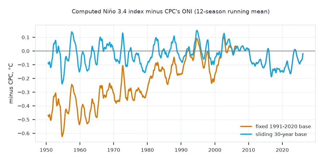
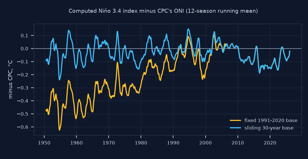
CPC computes ONI against 30-year base periods that it updates every five years, so early decades are not judged against today's warmer normals. Compare a single fixed 1991–2020 base with a sliding one centred on each year, against CPC, over the whole record:

def sliding(series):
    out = pd.Series(index=series.index, dtype=float)
    for y in range(series.index.year.min(), series.index.year.max() + 1):
        a, b = max(y - 15, 1950), min(y + 14, 2020)
        if b - a < 29:
            a, b = (1950, 1979) if y < 1965 else (1991, 2020)
        base = series[str(a):str(b)]
        m = base.groupby(base.index.month).mean()
        yr = series[str(y)]
        out[yr.index] = yr.values - yr.index.month.map(m).values
    return out.rolling(3, center=True).mean()
for label, idx in (("fixed 1991-2020", oni), ("sliding 30-year", sliding(n34))):
    d = (idx - CPC).dropna()
    print(f"{label:>16}: mean difference from CPC {d.mean():+.3f} °C, mean absolute {d.abs().mean():.3f} °C; 1950s mean {d['1950':'1959'].mean():+.2f} °C")

 fixed 1991-2020: mean difference from CPC -0.192 °C, mean absolute 0.211 °C; 1950s mean -0.42 °C
 sliding 30-year: mean difference from CPC -0.031 °C, mean absolute 0.088 °C; 1950s mean -0.04 °C

A sliding 30-year base reproduces CPC much more closely: a mean difference of -0.031 °C and a mean absolute difference of 0.088 °C, against 0.211 °C for the fixed base. The difference is concentrated in the early record: the 1950s come out 0.42 °C cooler with the fixed base and 0.04 °C with the sliding one.

Why the Nino 3.4 region

The Niño 3.4 region straddles the central and eastern equatorial Pacific, where changes in sea surface temperature during El Niño and La Niña are largest and most closely tied to the shift in tropical rainfall that drives their global effects. A monthly mean there would be noisy; the three-month running mean filters out short excursions, and the five-season persistence rule separates episodes from single warm or cool months. Anomalies, not temperatures, are what matter: the region's seasonal cycle is about 2 °C, so the same temperature can be normal in one month and anomalous in another.

The base period is the subtle part. The tropical Pacific has warmed since 1950, so anomalies against a recent base make the 1950s look cooler, and La Niña more frequent, than they were judged at the time. CPC's solution is a base that moves through the record; a fixed modern base is simpler but answers a different question. Either way, the ONI is an index of a state, not a forecast: CPC's announcements also weigh the atmosphere's response before declaring conditions.

Other regions, box edges and recent months

• Other Niño regions: Niño 1+2, Niño 3 and Niño 4 cover other parts of the equatorial Pacific; CPC's monthly sstoi.indices file lists all four.
• Box edges: whether the half-in cells at 5°S and 5°N are kept changes the mean slightly; state which cells were used.
• Order of operations: average the box, then take anomalies, then smooth; the reverse orders give nearly the same numbers here, but not with missing data.
• Time stamps: on this ERDDAP server ERSST months are stamped on the 1st until 2007 and on the 15th from 2008; without normalising to months, a join with CPC's table silently drops everything after 2007.
• Recent months: ERSST's latest month is preliminary and can change at the next update.

Internal links

• Sea surface temperature explained — ERSST and OISST compared
• How to download NOAA OISST sea surface temperature in Python — the daily product
• Fixing sea surface temperature anomalies that disagree between sources — why base periods matter

FAQ

How is the Oceanic Niño Index calculated?

As the three-month running mean of ERSST v5 sea surface temperature anomalies in the Niño 3.4 region, 5°S to 5°N and 170°W to 120°W, with anomalies relative to 30-year base periods that CPC updates every five years.

What ONI value means El Niño?

+0.5 °C or more for at least five consecutive overlapping three-month seasons; La Niña is -0.5 °C or less for the same length.

Can I compute the ONI in Python?

Yes: download ERSST for the box, average with cosine-of-latitude weights, subtract monthly base-period means and take a centred three-month mean; step 2 compares the result with CPC's values.

Is there an El Niño in 2026?

CPC's ONI for the most recent seasons in the table used on this page is printed in the quick answer; the index has been rising through 2026.