
How to extract phenology metrics from an NDVI time series
Problem statement
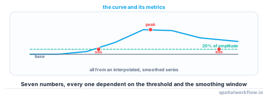
The metrics are simple to define and sensitive to every choice around them. Start of season, peak, end of season, length and integral are all read off a curve — and the curve is an interpolation through irregular, cloud-limited observations, smoothed by a window you chose, thresholded at a level you chose.
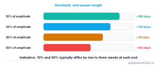
On a real Sentinel-2 series over Dutch arable land, 21 usable dates spanned 7 March to 6 September with gaps of 20 and 43 days, and the field-median NDVI ran 0.245 → 0.776 → 0.608. The metrics from that series are defensible. The same metrics with a 50% threshold instead of 20% are different by around a fortnight at each end, and neither number is wrong.
Quick answer
import numpy as np, pandas as pd

def phenology(dates, values, threshold=0.2, smooth_days=15):
    s = (pd.Series(values, index=pd.DatetimeIndex(dates))
         .reindex(pd.date_range(min(dates), max(dates), freq="D"))
         .interpolate("time")
         .rolling(smooth_days, center=True, min_periods=smooth_days // 3).mean()
         .dropna())

    base, peak = float(s.min()), float(s.max())
    amp = peak - base
    peak_date = s.idxmax()
    level = base + threshold * amp
    rising = s[(s >= level) & (s.index <= peak_date)]
    falling = s[(s >= level) & (s.index >= peak_date)]

    return {"base": round(base, 3), "peak": round(peak, 3),
            "amplitude": round(amp, 3), "peak_date": str(peak_date.date()),
            "sos": str(rising.index.min().date()) if len(rising) else None,
            "eos": str(falling.index.max().date()) if len(falling) else None,
            "integral": round(float((s - base).clip(lower=0).sum()), 1),
            "threshold": threshold, "smooth_days": smooth_days,
            "observations": int(np.isfinite(values).sum())}
Returning the threshold, the smoothing window and the observation count inside the result is the point: without them the metrics cannot be compared with anyone else's, including your own from last year.
Step-by-step solution
1. Build the series per field
Field medians are far less noisy than pixel series and the field is the management unit. Use pixel series only where within-field variation is the question.
2. Screen the observations before interpolating
Cloud, shadow and snow all produce valid-looking index values. A scene classification mask and a minimum clear fraction per date are the cheapest screen; on the reference series that removed 2 of 21 dates at a 60% threshold.
3. Interpolate onto a daily grid
Linear interpolation in time is adequate for most work. The important part is that every metric is computed from a regular grid, so a gap does not silently become a feature.
4. Smooth, and report the window
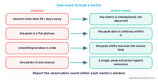
A 15-day centred rolling mean removes observation noise. It also shifts the peak of an asymmetric curve by roughly half the window, which is a systematic bias that belongs in the documentation.
5. Choose a threshold definition
Relative to amplitude (20% is common), absolute (NDVI 0.3), or the maximum of the derivative. Relative thresholds transfer between crops; absolute ones are easier to explain; the derivative maximum is the most physically meaningful and the noisiest.
6. Handle the double peak
Cover crops, cut grassland and catch crops give two peaks. A single-peak extractor reports a season running from the first green-up to the last senescence, which is not a season.
7. Report the evidence behind each metric
How many clear observations fall within ten days of the start of season, the peak and the end. A metric interpolated across a 43-day gap deserves less confidence than one bracketed by observations three days apart.
Code examples
Example 1 — the real series, and the metrics from it
import pandas as pd

season = pd.read_csv("season.csv", parse_dates=["date"])
usable = season[season.clear_frac > 0.6]
print(f"{len(usable)} usable dates of {len(season)}")
print(usable[["date", "ndvi_med", "ndre_med"]].to_string(index=False))

print(phenology(usable.date, usable.ndvi_med))
print(phenology(usable.date, usable.ndre_med))
19 usable dates of 21
date ndvi_med ndre_med
2025-03-07 0.245 0.151
2025-04-06 0.238 0.184
2025-05-13 0.400 0.279
2025-06-12 0.776 0.543
2025-06-30 0.774 0.514
2025-08-19 0.654 0.388
2025-09-06 0.608 0.385
Running the same function on NDVI and on NDRE is worth doing: the NDVI curve is flat at the top between 12 and 30 June, so its peak date is poorly determined, while the NDRE curve retains a peak.
Example 2 — the evidence behind each metric
import numpy as np, pandas as pd

def metric_support(dates, metric_date, window_days=10):
    d = pd.DatetimeIndex(dates)
    m = pd.Timestamp(metric_date)
    within = np.abs((d - m).days) <= window_days
    gaps = np.diff(np.sort(d)).astype("timedelta64[D]").astype(int)
    before = d[d <= m].max() if (d <= m).any() else None
    after = d[d >= m].min() if (d >= m).any() else None
    return {"observations_within": int(within.sum()),
            "days_to_previous": (m - before).days if before is not None else None,
            "days_to_next": (after - m).days if after is not None else None,
            "largest_gap_days": int(gaps.max()) if len(gaps) else None}

m = phenology(usable.date, usable.ndvi_med)
for key in ("sos", "peak_date", "eos"):
    print(key, m[key], metric_support(usable.date, m[key]))
An end of season bracketed by observations 43 days apart is an interpolation, and saying so is more useful than a confidence interval nobody believes.
Example 3 — a double-peak-aware extractor
import numpy as np, pandas as pd
from scipy.signal import find_peaks

def seasons(dates, values, threshold=0.2, smooth_days=15, min_prominence=0.1,
            min_separation_days=45):
    s = (pd.Series(values, index=pd.DatetimeIndex(dates))
         .reindex(pd.date_range(min(dates), max(dates), freq="D"))
         .interpolate("time")
         .rolling(smooth_days, center=True, min_periods=smooth_days // 3).mean()
         .dropna())

    base, amp = float(s.min()), float(s.max() - s.min())
    idx, props = find_peaks(s.values, prominence=min_prominence * amp,
                            distance=min_separation_days)
    if len(idx) == 0:
        return []

    out = []
    level = base + threshold * amp
    for i, p in enumerate(idx):
        left = s.index[:p][s.values[:p] < level]
        right = s.index[p:][s.values[p:] < level]
        out.append({
            "peak_date": str(s.index[p].date()),
            "peak": round(float(s.values[p]), 3),
            "prominence": round(float(props["prominences"][i]), 3),
            "sos": str(left.max().date()) if len(left) else None,
            "eos": str(right.min().date()) if len(right) else None,
        })
    return out
prominence is the parameter that separates a genuine second crop from a wobble in the senescence curve. Setting it as a fraction of the seasonal amplitude makes it transfer between fields and indices.
Explanation
Why interpolation is not optional
Metrics computed from the observations alone are metrics about when the sky was clear. With a 43-day gap over senescence, the "last date above the threshold" is whichever cloud-free date happened to fall before the gap. Interpolating onto a daily grid makes the metric a property of the curve, which is at least a consistent thing to compare between fields.
Why smoothing shifts the peak
A centred rolling mean is symmetric, so on a symmetric curve it leaves the peak in place. A crop curve is not symmetric — green-up is faster than senescence — so the mean pulls the peak towards the slower side by roughly half the window for a strongly asymmetric curve. The bias is systematic and therefore comparable between fields, provided the window is the same.
Why relative thresholds transfer and absolute ones do not
An absolute NDVI threshold of 0.3 is early emergence for maize and mid-season for a thin grassland. A threshold at 20% of the field's own amplitude adapts to the crop and the soil background, which is what makes it usable across a mixed farm. The cost is that a field with a small amplitude gets a threshold close to its noise floor.
Why the peak date is unreliable with NDVI
Between 12 and 30 June the reference series sat at 0.770–0.776. Any peak-finding on that plateau is picking between values separated by less than the measurement noise, so the peak date is effectively arbitrary within an eighteen-day window. A red-edge index has a real maximum in the same period.
Edge cases or notes
- Winter crops span the year end. Define the season window explicitly.
- Perennials never reach a low base. Amplitude-relative thresholds fail on orchards.
- Snow gives negative values. Mask rather than interpolating across.
- Series must be sorted. Duplicated dates break the interpolation.
- A partial series has no peak. Require coverage before and after.
- Savitzky–Golay and double-logistic fits impose a shape; the shape is an assumption.
- The integral is the most robust metric and the least interpretable.
- Report the observation count alongside every metric.
Internal links
- Crop phenology and growing seasons explained — what the metrics mean
- Vegetation indices explained: NDVI, EVI, NDRE and when each fails — why the NDVI peak is unreliable
- How to classify crop types from a satellite time series — the main consumer
- Growing degree days explained — expressing the metrics in thermal time
- How to build an NDVI time series for a polygon in Python — assembling the series
- How to resample a time series in xarray — the gridded equivalent
- How to mask clouds in Sentinel-2 imagery in Python — screening the dates
- NDVI stops responding in a dense canopy — the flat peak
FAQ
What phenology metrics should I extract?
Start of season, peak value and date, end of season, length, amplitude and the integral. The integral is the most robust and the least interpretable.
Do I have to interpolate the series?
Yes. Metrics computed from raw observations are metrics about when the sky was clear — a real series had a 43-day gap over senescence.
What threshold defines the start of season?
Whatever you publish. Twenty per cent of the seasonal amplitude is common and transfers between crops better than an absolute value.
Does smoothing bias the metrics?
It shifts the peak of an asymmetric curve by roughly half the window. The bias is systematic, so it is comparable as long as the window is fixed.
Why is my peak date unstable?
NDVI saturation. A real series sat between 0.770 and 0.776 for eighteen days, so the peak date within that window is arbitrary.
How do I handle two crops in one season?
Use a peak finder with a prominence threshold expressed as a fraction of the seasonal amplitude, and return one set of metrics per peak.