
Population Grid Accuracy Explained
On this page
Problem statement
"How accurate is this population grid?" has no single answer. A modelled grid can match a country's population to a tenth of a percent and get most of its 1 km cells wrong by half; it can be excellent for municipalities that existed when its inputs were made and poor for ones merged since. Accuracy depends on the size of the area being estimated, on how the grid was made, and on what it is compared with. Knowing which of those dominates tells a user how large an area must be before the grid can be trusted.
This page measures the accuracy of GHS-POP and WorldPop against Statistics Netherlands' census grid at a range of scales, from 1 km cells to 20 km cells and circles around sample points, and explains where the errors come from.
Quick answer
Aggregate the models and the census to square cells of increasing size and compare:
for size in (1, 2, 5, 10, 20):
    K = agg(size)
    print(f"{size:>3} km cells: {len(K):>6,}  " + "   ".join(
        f"{m} median |error| {((K[m] - K.census).abs() / K.census).median():>5.1%}" for m in ("ghs_pop", "worldpop")))
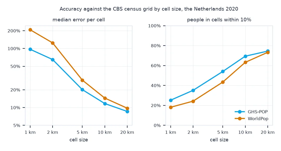
1 km cells: 23,556 ghs_pop median |error| 97.0% worldpop median |error| 207.7%
2 km cells: 8,211 ghs_pop median |error| 65.1% worldpop median |error| 124.5%
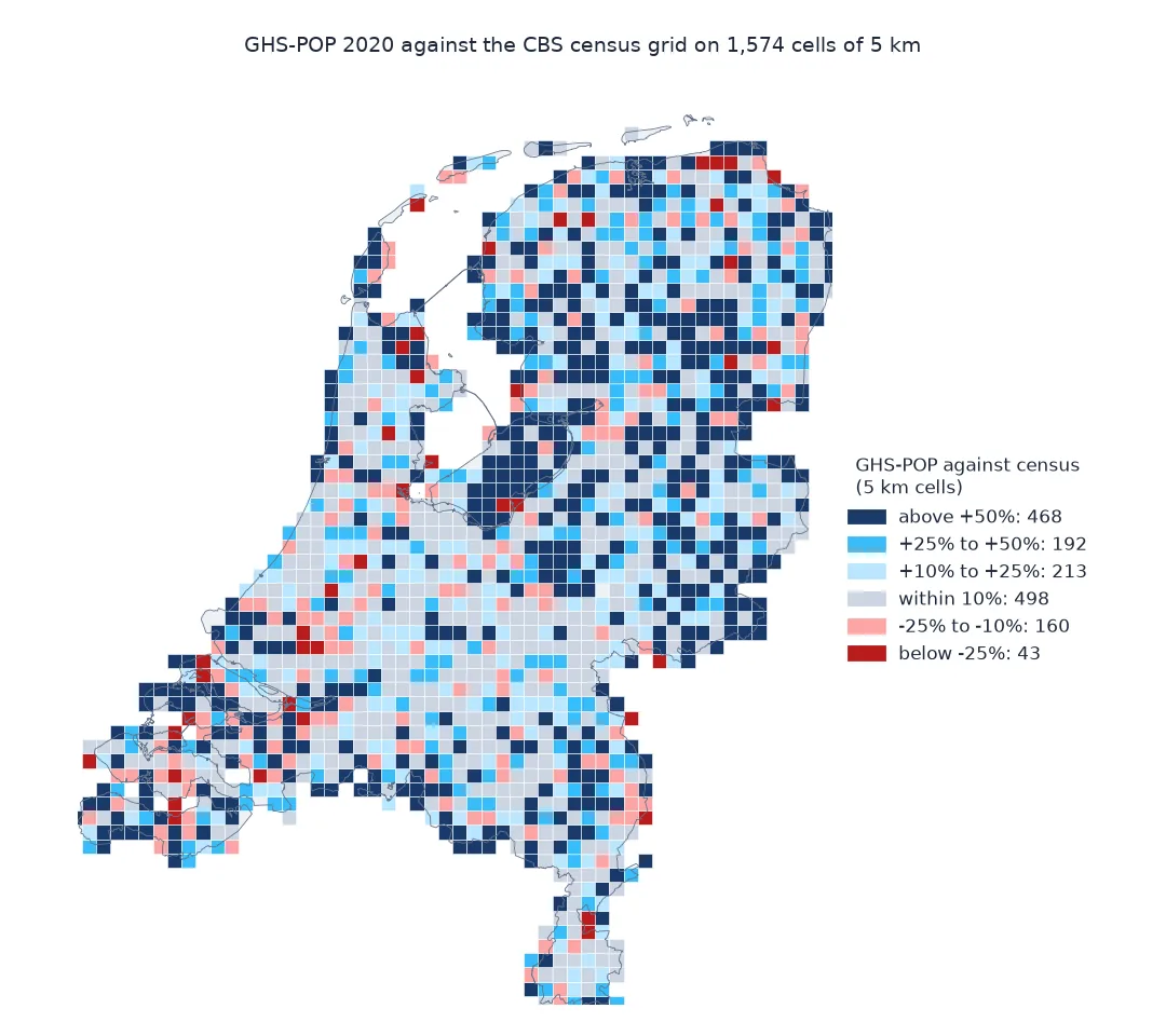
5 km cells: 1,574 ghs_pop median |error| 20.1% worldpop median |error| 29.2%
10 km cells: 447 ghs_pop median |error| 11.7% worldpop median |error| 14.5%
20 km cells: 132 ghs_pop median |error| 8.6% worldpop median |error| 9.8%
At 1 km the median cell is off by 97% in GHS-POP and 208% in WorldPop: most 1 km cells are nearly empty, and a few dozen people too many doubles them. The error falls fast with scale, to about 20% to 30% at 5 km and 9% to 10% at 20 km, where only 132 cells are left.
Error by scale, random against systematic, circles around points
1. Error by scale, weighted by people
A median over cells treats a farm cell like a city cell. Weight by people instead: what share of the population lives in cells the model gets within 10%?
for size in (1, 2, 5, 10, 20):
    K = agg(size)
    ok = {m: (((K[m] - K.census).abs() / K.census) <= 0.10) for m in ("ghs_pop", "worldpop")}
    print(f"{size:>3} km: people in cells within 10%: GHS-POP {K.census[ok['ghs_pop']].sum() / K.census.sum():.0%}, "
          f"WorldPop {K.census[ok['worldpop']].sum() / K.census.sum():.0%}")
1 km: people in cells within 10%: GHS-POP 25%, WorldPop 18%
2 km: people in cells within 10%: GHS-POP 35%, WorldPop 24%
5 km: people in cells within 10%: GHS-POP 54%, WorldPop 43%
10 km: people in cells within 10%: GHS-POP 69%, WorldPop 63%
20 km: people in cells within 10%: GHS-POP 74%, WorldPop 73%
Weighted by people the picture is kinder, because populous cells are estimated better. Even so, at 1 km only a quarter of people live in cells GHS-POP gets within 10%, and a fifth for WorldPop; at 5 km about half; at 20 km three quarters, with the gains slowing between 10 and 20 km.
2. Random error and systematic error
Aggregation cancels errors that go both ways, but not errors that go the same way everywhere. Compare each model's total in dense and sparse 5 km cells with the census:
K = agg(5)
K["kind"] = np.where(K.census / 25 >= 1_000, "5 km cells over 1,000 per km2", "5 km cells under 1,000 per km2")
print(K.groupby("kind")[["census", "ghs_pop", "worldpop"]].sum().assign(
    ghs_pop_vs_census=lambda t: t.ghs_pop / t.census - 1, worldpop_vs_census=lambda t: t.worldpop / t.census - 1).to_string(
    formatters={"census": "{:,.0f}".format, "ghs_pop": "{:,.0f}".format, "worldpop": "{:,.0f}".format,
                "ghs_pop_vs_census": "{:+.1%}".format, "worldpop_vs_census": "{:+.1%}".format}))
census ghs_pop worldpop ghs_pop_vs_census worldpop_vs_census
kind
5 km cells over 1,000 per km2 9,682,085 9,321,330 9,141,176 -3.7% -5.6%
5 km cells under 1,000 per km2 7,058,700 8,041,439 8,404,067 +13.9% +19.1%
Summed over all dense 5 km cells, GHS-POP has 3.7% too few people and WorldPop 5.6% too few; over all sparse ones, 13.9% and 19.1% too many. These are totals over millions of people, so they are not noise that more aggregation would remove: both models move people from dense to sparse land.
3. Circles around points
Most analyses ask about a buffer, not a grid cell. Draw 300 sample points from the census residents, weighted by population, and compare each model's total within circles of increasing radius:
rng = np.random.default_rng(0)
idx = rng.choice(len(CBS_POP), 300, replace=False, p=CBS_POP / CBS_POP.sum())
trees = {k: cKDTree(xy) for k, (xy, _) in SRC.items()}
for r in (500, 1_000, 2_000, 5_000):
    tot = {k: np.array([SRC[k][1][trees[k].query_ball_point(CBS_XY[i], r)].sum() for i in idx]) for k in SRC}
    e = {m: np.median(np.abs(tot[m] / tot["census"] - 1)) for m in ("ghs_pop", "worldpop")}
    print(f"radius {r / 1000:>3.1f} km: median census population {np.median(tot['census']):>8,.0f}; median |error| GHS-POP {e['ghs_pop']:.1%}, WorldPop {e['worldpop']:.1%}")
radius 0.5 km: median census population 3,268; median |error| GHS-POP 22.5%, WorldPop 31.7%
radius 1.0 km: median census population 9,255; median |error| GHS-POP 14.8%, WorldPop 23.0%
radius 2.0 km: median census population 23,245; median |error| GHS-POP 10.7%, WorldPop 15.0%
radius 5.0 km: median census population 84,072; median |error| GHS-POP 6.3%, WorldPop 6.5%
Around 300 points drawn where people live, a 500 m circle holds a median of 3,268 residents, and the models are typically 23% and 32% off. At 1 km the errors are 15% and 23%, at 2 km 11% and 15%, and at 5 km, with a median of 84,072 residents, about 6% for both.
How big an area needs to be
The data used on this page
The CBS 100 m grid, final 2020 edition, as the reference; GHS-POP R2023A epoch 2020 at 100 m in Mollweide (tiles R3_C19 and R4_C19); WorldPop R2025A constrained 2020; and the land boundary from the PDOK CBS gebiedsindelingen web feature service.
import io
import zipfile
from pathlib import Path

import geopandas as gpd
import numpy as np
import pandas as pd
import pyogrio
import rasterio
import requests
from pyproj import Transformer
from rasterio.features import geometry_mask
from rasterio.merge import merge
from scipy.spatial import cKDTree

Path("data").mkdir(exist_ok=True)
GPKG = Path("data/cbs_vk100_2020_vol.gpkg")
if not GPKG.exists():
    url = "https://www.cbs.nl/-/media/cbs/dossiers/nederland-regionaal/vierkanten/100/2023-cbs_vk100_2020_vol.zip"
    zipfile.ZipFile(io.BytesIO(requests.get(url, timeout=900).content)).extract(GPKG.name, "data")
WP = Path("data/nld_pop_2020_CN_100m_R2025A_v1.tif")
if not WP.exists():
    WP.write_bytes(requests.get("https://data.worldpop.org/GIS/Population/Global_2015_2030/R2025A/2020/NLD/v1/100m/constrained/"
                                "nld_pop_2020_CN_100m_R2025A_v1.tif", timeout=600).content)
BASE = "https://jeodpp.jrc.ec.europa.eu/ftp/jrc-opendata/GHSL/GHS_POP_GLOBE_R2023A/GHS_POP_E2020_GLOBE_R2023A_54009_100/V1-0/tiles"
srcs = []
for t in ("R3_C19", "R4_C19"):
    tif = Path("data", f"GHS_POP_E2020_GLOBE_R2023A_54009_100_V1_0_{t}.tif")
    if not tif.exists():
        zipfile.ZipFile(io.BytesIO(requests.get(f"{BASE}/{tif.stem}.zip", timeout=900).content)).extract(tif.name, "data")
    srcs.append(rasterio.open(tif))
B = Path("data/landsdeel_2020.geojson")
if not B.exists():
    B.write_bytes(requests.get("https://service.pdok.nl/cbs/gebiedsindelingen/2020/wfs/v1_0", timeout=300, params={
        "service": "WFS", "version": "2.0.0", "request": "GetFeature", "typeName": "gebiedsindelingen:landsdeel_gegeneraliseerd",
        "outputFormat": "application/json", "srsName": "EPSG:28992"}).content)
NL = gpd.read_file(B).dissolve()
def cells(a, transform, crs):
    inside = ~geometry_mask(NL.to_crs(crs).geometry, a.shape, transform)
    r, c = np.nonzero(inside & (a > 0))
    x, y = rasterio.transform.xy(transform, r, c)
    X, Y = Transformer.from_crs(crs, 28992, always_xy=True).transform(np.asarray(x), np.asarray(y))
    return np.c_[X, Y], a[r, c].astype("float64")
g, gt = merge(srcs, bounds=(230_000, 5_930_000, 530_000, 6_280_000))
GHS_XY, GHS_POP = cells(g[0], gt, "ESRI:54009")
with rasterio.open(WP) as src:
    WP_XY, WP_POP = cells(src.read(1), src.transform, src.crs)
V = pyogrio.read_dataframe(GPKG, columns=["crs28992res100m", "aantal_inwoners"], read_geometry=False)
V = V[V.aantal_inwoners > 0]
CBS_XY = V.crs28992res100m.str.extract(r"E(\d+)N(\d+)").astype(int).to_numpy() * 100 + 50
CBS_POP = V.aantal_inwoners.to_numpy("float64")
SRC = {"census": (CBS_XY, CBS_POP), "ghs_pop": (GHS_XY, GHS_POP), "worldpop": (WP_XY, WP_POP)}
def agg(size_km):
    """Sum each source into RD New squares of size_km; keep squares where the census has residents."""
    f = size_km * 1000
    K = pd.concat({k: pd.Series(p).groupby([xy[:, 0] // f, xy[:, 1] // f]).sum() for k, (xy, p) in SRC.items()}, axis=1).fillna(0)
    return K[K.census > 0]
print(f"census {CBS_POP.sum():,.0f}; GHS-POP {GHS_POP.sum():,.0f}; WorldPop {WP_POP.sum():,.0f} people inside the land boundary")
census 16,740,785; GHS-POP 17,418,265; WorldPop 17,589,165 people inside the land boundary
Inside the land boundary the census holds 16,740,785 residents, GHS-POP 17,418,265 and WorldPop 17,589,165.
Example 1: how big an area needs to be
Turn the scale results into a rule of thumb: the smallest square cell at which half of each model's cells are within 10% of the census:
for m in ("ghs_pop", "worldpop"):
    for size in (1, 2, 5, 10, 20, 40):
        K = agg(size)
        share = (((K[m] - K.census).abs() / K.census) <= 0.10).mean()
        if share >= 0.5:
            print(f"{m}: half of all cells within 10% from {size} km cells upward ({share:.0%} of {len(K):,} cells)")
            break
    else:
        print(f"{m}: not reached by 40 km cells")
ghs_pop: half of all cells within 10% from 20 km cells upward (60% of 132 cells)
worldpop: half of all cells within 10% from 20 km cells upward (52% of 132 cells)
Square cells need to be 20 km on a side before half of them are within 10% of the census, for either model; circles reach similar accuracy sooner, because points drawn where people live sit in populated places that the models estimate better.
Three sources of modelled error
A modelled grid's error has three main sources. The inputs: the census units the model starts from, their size, and their year. GHS-POP's Dutch inputs are 418 municipalities in 2011, carried to 2020 by growth rates; anything that changed inside a municipality since then is invisible to it. The model: what it uses to spread people inside a unit, and how well that predicts residents. Built-up area and volume say where buildings are, not how many people live in each, so the models put too many people where buildings are sparse and too few where they are full. And the comparison: what the grid is checked against, at what scale, and with what geometry; WorldPop's large municipal errors in the zonal sum guide came from boundaries, not from its model.
Scale is the lever a user controls. Random errors, a few people too many here and too few there, cancel as cells are summed, so the typical error falls quickly with area. Systematic errors, the same direction across a whole class of places, do not cancel: no amount of aggregation removes a model's tendency to understate dense districts, only an area large enough to mix dense and sparse land. The practical rule is to evaluate a grid at the scale of the question, and to treat cell-level values from a modelled grid as a smooth estimate rather than a count.
Reference errors and resolution
- The reference has errors too: the census grid is rounded down and short of the official total; where differences are a few people per cell, both grids are within each other's noise.
- Other countries: the Netherlands has small census units and a dense address register; where a model's inputs are large districts from an old census, its errors are larger at every scale.
- Relative and absolute error: percentage errors explode in nearly empty cells; report absolute errors or weight by population alongside.
- Resolution is not accuracy: a 100 m model cell is not more accurate than a 1 km one; it is the same estimate at a finer grain.
Internal links
- How to compare population grids cell by cell in Python — the 1 km comparison in detail
- Population grids explained — how each grid is made
- How to sum a population grid by municipality in Python — errors by administrative area
FAQ
How accurate are gridded population datasets?
It depends on the area: for the Netherlands in 2020, the median 1 km cell of GHS-POP is off by 97% against the census, a 20 km cell by 8.6%, and a 5 km circle around where people live by about 6%.
Why are modelled population grids less accurate in cities?
They spread people by what satellites see, which captures where buildings are but not how many people live in each, so dense housing is understated.
What area should I aggregate a population grid to?
To the scale of the question, and large enough that the grid's error at that scale, measured against a census where one exists, is acceptable; the Example on this page gives the cell size at which half the cells are within 10%.
Is a finer population grid more accurate?
Not by itself: a finer modelled grid is the same estimate at a smaller cell size, and its errors per cell are larger.