Fixing Population Densities That Are Wrong on Latitude-Longitude Grids

Problem statement

Densities computed from a population grid in latitude and longitude come out too low, or too high, by the same factor everywhere in one country and by different factors in countries at different latitudes. Two mistakes cause it. The first divides every cell by one area, 1 km² because the grid is "1 km", or the equatorial area of a 30 arc-second cell. The second takes polygon areas with .area in EPSG:4326, which returns square degrees, not square kilometres, and a square degree shrinks towards the poles.

This page reproduces both mistakes on GHS-POP 2020, measures the error at every latitude of the tile, shows how it biases comparisons between cities, and fixes it with geodesic or equal-area areas.

Quick answer

Divide each row by its own geodesic area, and take polygon areas in an equal-area CRS:

row_km2 = np.array([abs(geod.polygon_area_perimeter([0, res, res, 0], [la, la, la + tf.e, la + tf.e])[0]) / 1e6 for la in lats])
for label, area in (("1 km2 per cell", 1.0), ("equatorial cell, 0.855 km2", 0.855), ("geodesic area per row", row_km2[:, None])):
    d = NLPOP / np.broadcast_to(area, NLPOP.shape)
    print(f"{label:>28}: densest cell {d.max():>7,.0f}, country {NLPOP.sum() / np.broadcast_to(area, NLPOP.shape)[~NLPOP.mask].sum():>4,.0f} per km2")

              1 km2 per cell: densest cell  11,407, country  262 per km2
  equatorial cell, 0.855 km2: densest cell  13,342, country  306 per km2
       geodesic area per row: densest cell  21,534, country  496 per km2

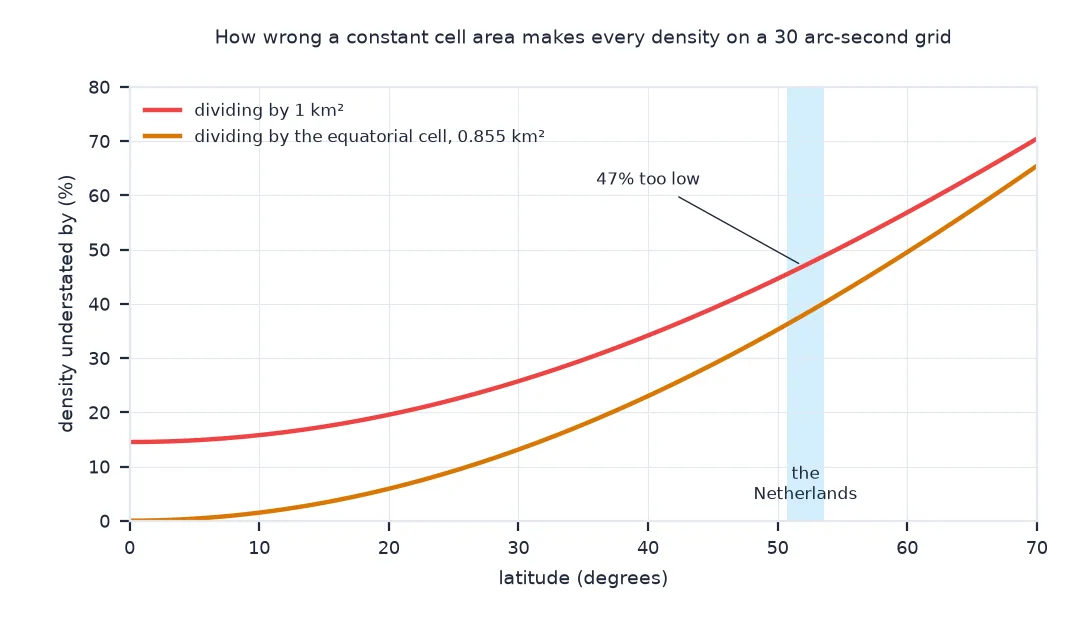
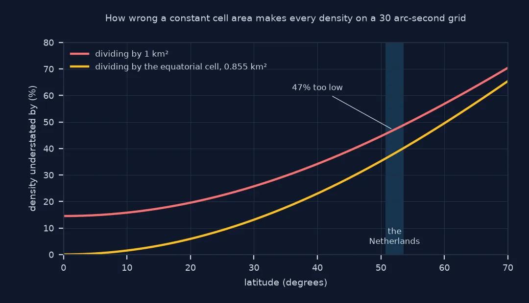
Dividing by 1 km² gives the Netherlands 262 people per km² and its densest cell 11,407; dividing by the equatorial cell area gives 306 and 13,342. With each row's own area the figures are 496 and 21,534: the constants understate every Dutch density by 47% and 38%.

The error by latitude, square degrees, a biased comparison

1. The error at every latitude

The ratio of the true cell area to the assumed one is the factor by which every density is wrong. Across the tile, from northern France to southern Norway:

for la in (49.1, 52.0, 55.0, 59.0):
    i = int((T.f - la) / res)
    print(f"{la:>4} N: cell {row_km2_tile[i]:.3f} km2; dividing by 1 km2 understates density by {1 - row_km2_tile[i]:.0%}, "
          f"by the equatorial cell by {1 - row_km2_tile[i] / 0.855:.0%}")

49.1 N: cell 0.564 km2; dividing by 1 km2 understates density by 44%, by the equatorial cell by 34%
52.0 N: cell 0.531 km2; dividing by 1 km2 understates density by 47%, by the equatorial cell by 38%
55.0 N: cell 0.495 km2; dividing by 1 km2 understates density by 51%, by the equatorial cell by 42%
59.0 N: cell 0.445 km2; dividing by 1 km2 understates density by 56%, by the equatorial cell by 48%

The error grows with latitude: at the tile's southern edge a cell is 0.564 km² and a 1 km² assumption understates density by 44%; at 59°N, 0.445 km² and 56%.

2. Square degrees from .area

geopandas computes .area in the units of the CRS. In EPSG:4326 those are square degrees:

deg2 = GM.to_crs(4326).area
km2 = GM.to_crs(3035).area / 1e6
ratio = km2 / deg2
print(f"km2 per square degree across Dutch municipalities: {ratio.min():,.0f} to {ratio.max():,.0f}")
print(f"density of Amsterdam: {OFF['GM0363'] / deg2[GM.statcode == 'GM0363'].iloc[0]:,.0f} 'per square degree', "
      f"{OFF['GM0363'] / km2[GM.statcode == 'GM0363'].iloc[0]:,.0f} per km2")

km2 per square degree across Dutch municipalities: 7,387 to 7,847
density of Amsterdam: 33,645,671 'per square degree', 4,440 per km2

Across Dutch municipalities a square degree ranges from 7,387 to 7,847 km², depending on latitude. Divided by its area in square degrees, Amsterdam has 33.6 million people "per square degree"; divided by its area in km², measured in EPSG:3035, 4,440 per km².

3. A biased comparison between cities

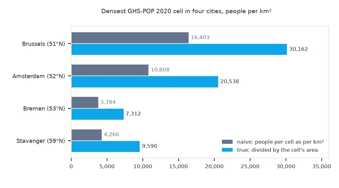
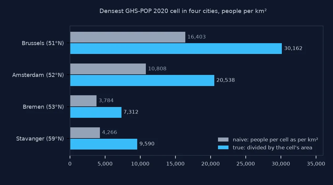
A single constant does not just scale every density; it scales them by different amounts at different latitudes. Compare the densest cell of four cities in the tile:

cities = {"Brussels": (4.35, 50.85), "Amsterdam": (4.9, 52.37), "Bremen": (8.8, 53.08), "Stavanger": (5.73, 58.97)}
with rasterio.open(GHS) as src:
    for name, (x, y) in cities.items():
        win = rasterio.windows.from_bounds(x - 0.1, y - 0.06, x + 0.1, y + 0.06, transform=src.transform)
        a = src.read(1, window=win, boundless=True, fill_value=0)
        r = np.unravel_index(a.argmax(), a.shape)[0] + int(win.row_off)
        print(f"{name:>10}: {a.max():>6,.0f} people in the densest cell; per km2 naive {a.max():>6,.0f}, true {a.max() / row_km2_tile[r]:>6,.0f}")

  Brussels: 16,403 people in the densest cell; per km2 naive 16,403, true 30,162
 Amsterdam: 10,808 people in the densest cell; per km2 naive 10,808, true 20,538
    Bremen:  3,784 people in the densest cell; per km2 naive  3,784, true  7,312
 Stavanger:  4,266 people in the densest cell; per km2 naive  4,266, true  9,590

The densest cell in the tile is in Brussels, with 16,403 people: 30,162 per km² on its true area, not 16,403. The constant also distorts comparisons: the naive figures put Stavanger 13% above Bremen, the true densities 31%, because Stavanger's cells, at 59°N, are 14% smaller than Bremen's at 53°N.

Checking the fix against an independent area

The data used on this page

GHS-POP R2023A epoch 2020 at 30 arc-seconds (tile R4_C19, 0° to 10°E and 49.1°N to 59.1°N, from Brussels to Stavanger), and the 2020 country and municipality boundaries from the PDOK CBS gebiedsindelingen web feature service with each municipality's population on 1 January 2020 from StatLine table 03759ned.

import io
import json
import zipfile
from pathlib import Path

import geopandas as gpd
import numpy as np
import rasterio
import requests
from pyproj import Geod
from rasterio.mask import mask

Path("data").mkdir(exist_ok=True)
name = "GHS_POP_E2020_GLOBE_R2023A_4326_30ss"
GHS = Path("data", f"{name}_V1_0_R4_C19.tif")
if not GHS.exists():
    url = f"https://jeodpp.jrc.ec.europa.eu/ftp/jrc-opendata/GHSL/GHS_POP_GLOBE_R2023A/{name}/V1-0/tiles/{GHS.stem}.zip"
    zipfile.ZipFile(io.BytesIO(requests.get(url, timeout=600).content)).extract(GHS.name, "data")
for layer in ("landsdeel", "gemeente"):
    path = Path("data", f"{layer}_2020.geojson")
    if not path.exists():
        path.write_bytes(requests.get("https://service.pdok.nl/cbs/gebiedsindelingen/2020/wfs/v1_0", timeout=300, params={
            "service": "WFS", "version": "2.0.0", "request": "GetFeature", "typeName": f"gebiedsindelingen:{layer}_gegeneraliseerd",
            "outputFormat": "application/json", "srsName": "EPSG:28992"}).content)
C = Path("data/cbs_pop_2020.json")
if not C.exists():
    C.write_bytes(requests.get("https://opendata.cbs.nl/ODataApi/odata/03759ned/TypedDataSet", timeout=300, params={
        "$filter": "Geslacht eq 'T001038' and Leeftijd eq '10000' and BurgerlijkeStaat eq 'T001019' and Perioden eq '2020JJ00' "
                   "and (substring(RegioS,0,2) eq 'GM' or substring(RegioS,0,2) eq 'NL')",
        "$select": "RegioS,BevolkingOp1Januari_1"}).content)
OFF = {r["RegioS"].strip(): r["BevolkingOp1Januari_1"] for r in json.loads(C.read_text())["value"] if r["BevolkingOp1Januari_1"]}
GM = gpd.read_file("data/gemeente_2020.geojson")
NL = gpd.read_file("data/landsdeel_2020.geojson").dissolve()
geod = Geod(ellps="WGS84")
with rasterio.open(GHS) as src:
    a, tf = mask(src, NL.to_crs(src.crs).geometry, crop=True, filled=False)
    T = src.transform; rows = src.height
NLPOP, res = a[0], tf.a
lats = tf.f + tf.e * np.arange(NLPOP.shape[0])
row_km2_tile = np.array([abs(geod.polygon_area_perimeter([0, res, res, 0], [la, la, la + T.e, la + T.e])[0]) / 1e6
                         for la in T.f + T.e * np.arange(rows)])
print(f"tile rows: {rows}; cell area {row_km2_tile[-1]:.3f} km2 at the bottom to {row_km2_tile[0]:.3f} km2 at the top")

tile rows: 1200; cell area 0.564 km2 at the bottom to 0.443 km2 at the top

The tile has 1,200 rows; a cell covers 0.564 km² in the bottom row and 0.443 km² in the top one.

Example 1: check the fix against an independent area

Sum the geodesic cell areas over the cells inside the country and compare with the land area of the same boundary measured in two projected CRSs:

cells_km2 = np.broadcast_to(row_km2[:, None], NLPOP.shape)[~NLPOP.mask].sum()
print(f"cells inside the boundary: {cells_km2:,.0f} km2")
print(f"boundary in EPSG:28992 (RD New): {NL.area.iloc[0] / 1e6:,.0f} km2; in EPSG:3035 (LAEA Europe): {NL.to_crs(3035).area.iloc[0] / 1e6:,.0f} km2")
print(f"cell count x 1 km2: {NLPOP.count():,} km2")

cells inside the boundary: 35,090 km2
boundary in EPSG:28992 (RD New): 35,085 km2; in EPSG:3035 (LAEA Europe): 35,087 km2
cell count x 1 km2: 66,493 km2

The geodesic areas of the 66,493 cells inside the boundary add up to 35,090 km², within 5 km² of the boundary's own area in RD New, 35,085 km², and in LAEA Europe, 35,087 km². Counting each cell as 1 km² would make the country 66,493 km², nearly twice its size.

A grid is only 1 km in one sense

A grid described as "1 km" or "30 arc-second" is only 1 km in one sense. Its cells are 30 arc-seconds of latitude tall, which is about 0.93 km everywhere, and 30 arc-seconds of longitude wide, which is 0.93 km at the equator and shrinks with the cosine of the latitude. Their area therefore depends on the row. Equal-area grids, such as the Mollweide versions of GHS-POP or national grids, have no such problem: every cell is the same area by construction.

The square-degree mistake is the same thing for polygons. geopandas does not convert units; .area on a layer in EPSG:4326 returns square degrees, and recent versions warn that the result is "likely incorrect" for a geographic CRS. Across Dutch municipalities a square degree ranges from 7,387 to 7,847 km², and it keeps shrinking towards the poles, so a density per square degree is not comparable between places and is not a density in any useful sense.

Ellipsoidal areas and mixed grids

• Area of a polygon on the ellipsoid: geod.geometry_area_perimeter(polygon) gives the geodesic area directly from coordinates in degrees, without choosing a projection.
• Which equal-area CRS: any equal-area projection gives the same areas to within rounding; EPSG:3035 for Europe, EPSG:6933 or ESRI:54009 globally. Web Mercator, EPSG:3857, is not one of them: at 52°N it inflates areas about 2.6 times.
• Mixing grids: resampling a latitude-longitude population grid onto an equal-area grid changes the cell areas but must not change the counts; see the reprojection fix.
• Very large areas: for continents the cell area also varies within a cell's height slightly; the per-row geodesic area already accounts for it.

Internal links

• How to map population density per km² from a population grid in Python — the density map done right
• How to Choose the Right Projected CRS for Your Study Area — areas in the right CRS
• Why density depends on the boundary — the other reason densities disagree

FAQ

Why is my population density too low?

Each cell was probably divided by 1 km² or by the equatorial cell area, when at 52°N a 30 arc-second cell covers 0.53 km²; divide each row by its own area.

Why does geopandas give tiny or huge areas?

The layer is in a geographic CRS such as EPSG:4326, so .area returns square degrees; reproject to an equal-area CRS before measuring.

Is a 30 arc-second grid 1 km?

Only near the equator; at 52°N its cells are 0.57 km wide, 0.93 km tall and 0.53 km² in area.

Does Web Mercator give correct areas?

No; it inflates areas by the square of 1 over the cosine of the latitude, about 2.6 times at 52°N.