
How to Compare Population Grids Cell by Cell in Python
On this page
Problem statement
Two modelled population grids, set against a census grid of registered residents square kilometre by square kilometre, miss the median populated cell by 74 and 120 people — in cells where the census counts 55. In the emptiest cells the models put four and six times too many people; in the densest, 13% to 23% too few. A correlation over all cells, 0.93 to 0.95 here, shows none of that, because any grid that puts more people in cities than in fields scores well on it.
Below, the 100 m census squares, GHS-POP at 100 m and WorldPop at 3 arc-seconds go onto one 1 km grid in RD New.
Quick answer
Assign every fine cell to a 1 km cell of one grid by its centre, sum, and align the three on the same index:
K = pd.concat({"census": km(CBS_XY, CBS_POP), "ghs_pop": km(GHS_XY, GHS_POP), "worldpop": km(WP_XY, WP_POP)}, axis=1).fillna(0)
K = K[K.census > 0]                                                       # compare where the census has residents
for m in ("ghs_pop", "worldpop"):
    e = K[m] - K.census
    print(f"{m:>8}: total {K[m].sum():,.0f} against {K.census.sum():,.0f}; "
          f"r = {np.corrcoef(K[m], K.census)[0, 1]:.3f}; median absolute error {e.abs().median():,.0f} people per km2")
ghs_pop: total 16,587,776 against 16,740,785; r = 0.945; median absolute error 74 people per km2
worldpop: total 16,634,547 against 16,740,785; r = 0.928; median absolute error 120 people per km2
On the 23,556 cells of 1 km where the census has residents, both models come within 1% of the census total and correlate at 0.93 to 0.95. The median cell is off by 74 people in GHS-POP and 120 in WorldPop, in cells whose median census population is 55.
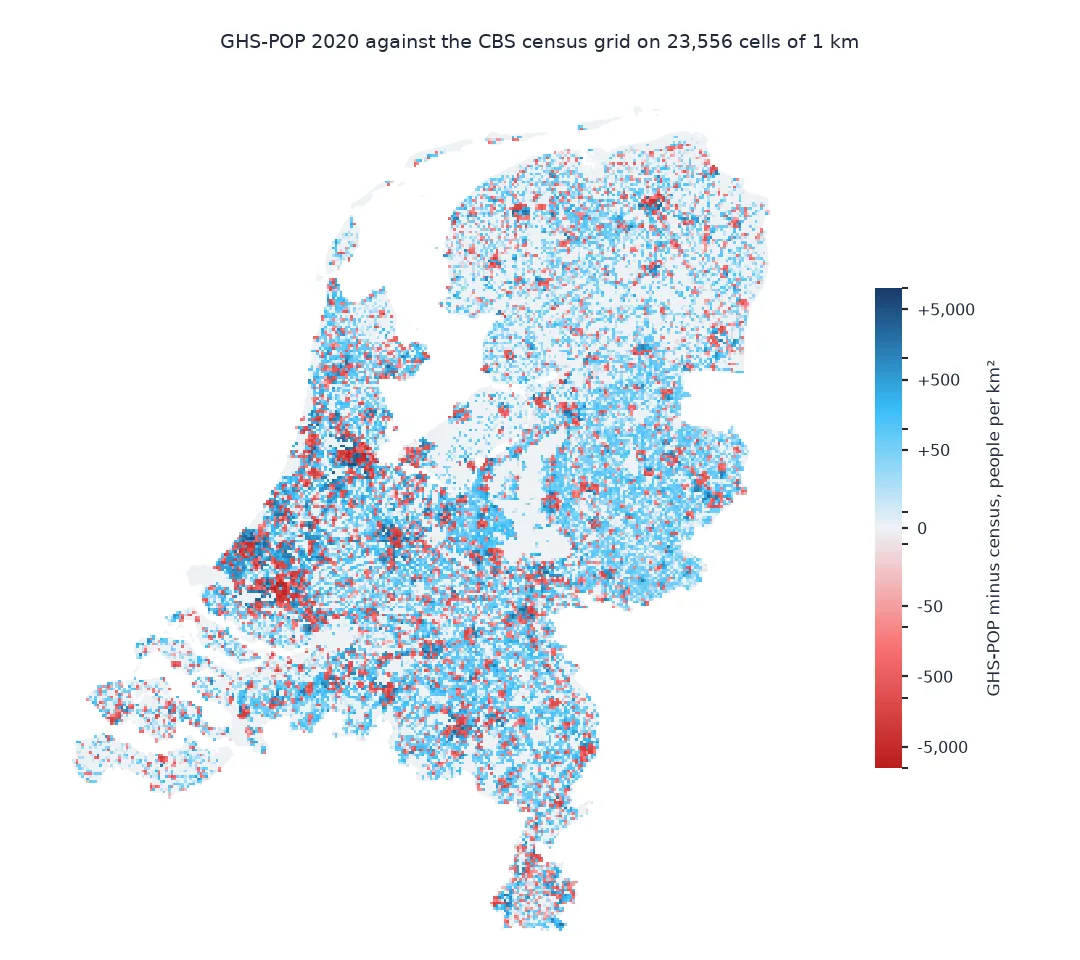
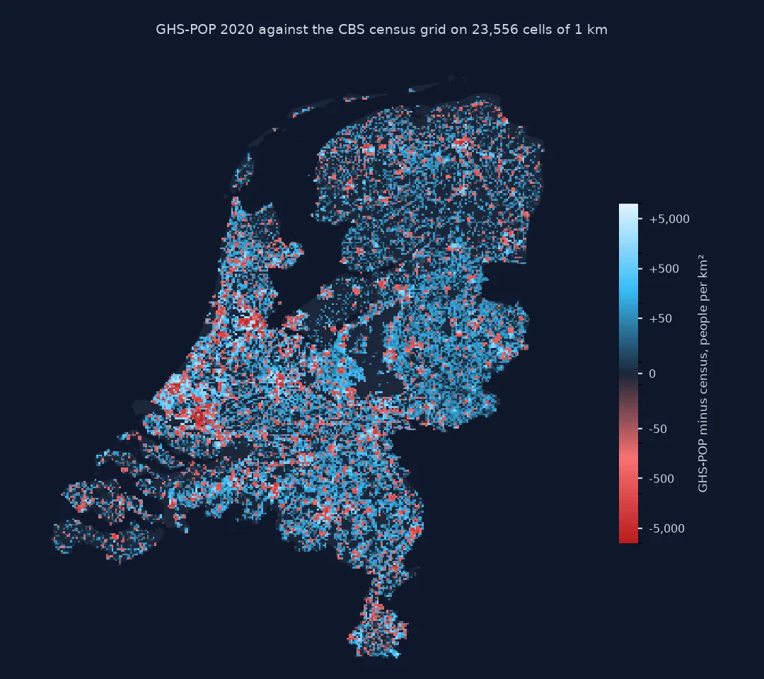
One grid for all, agreement, errors by density
1. One grid for all three
Each source has its own grid and CRS. Convert each fine cell's centre to RD New and floor to the kilometre; the census squares are already in RD New, so their IDs divide straight into kilometres:
print(f"census squares: {len(CBS_POP):,}; GHS-POP 100 m cells: {len(GHS_POP):,}; WorldPop cells: {len(WP_POP):,}")
print(f"1 km cells with census residents: {len(K):,}")
print(K.describe().loc[["mean", "50%", "max"]].round(0).to_string())
census squares: 379,905; GHS-POP 100 m cells: 1,221,963; WorldPop cells: 3,527,556
1 km cells with census residents: 23,556
census ghs_pop worldpop
mean 711.0 704.0 706.0
50% 55.0 140.0 211.0
max 23165.0 20804.0 11664.0
379,905 census squares, 1.2 million GHS-POP cells and 3.5 million WorldPop cells go into 23,556 populated 1 km cells. The means agree, about 710 people per cell, but the medians do not: 55 in the census, 140 in GHS-POP and 211 in WorldPop, and the densest cell holds 23,165 in the census, 20,804 in GHS-POP and 11,664 in WorldPop.
2. How often they agree
A correlation over all cells is dominated by the contrast between city and country. Ask instead what share of cells, and of people, each model gets within 25% of the census:
for m in ("ghs_pop", "worldpop"):
    rel = (K[m] - K.census) / K.census
    ok = rel.abs() <= 0.25
    print(f"{m:>8}: cells within 25%: {ok.mean():.0%}; people in those cells: {K.census[ok].sum() / K.census.sum():.0%}; "
          f"cells off by more than half: {(rel.abs() > 0.5).mean():.0%}")
ghs_pop: cells within 25%: 24%; people in those cells: 60%; cells off by more than half: 60%
worldpop: cells within 25%: 18%; people in those cells: 46%; cells off by more than half: 68%
Only a quarter of the cells are within 25% of the census in GHS-POP and under a fifth in WorldPop, and most cells are off by more than half. The cells that are right are the populous ones, so 60% and 46% of the people live in cells the models get within 25%.
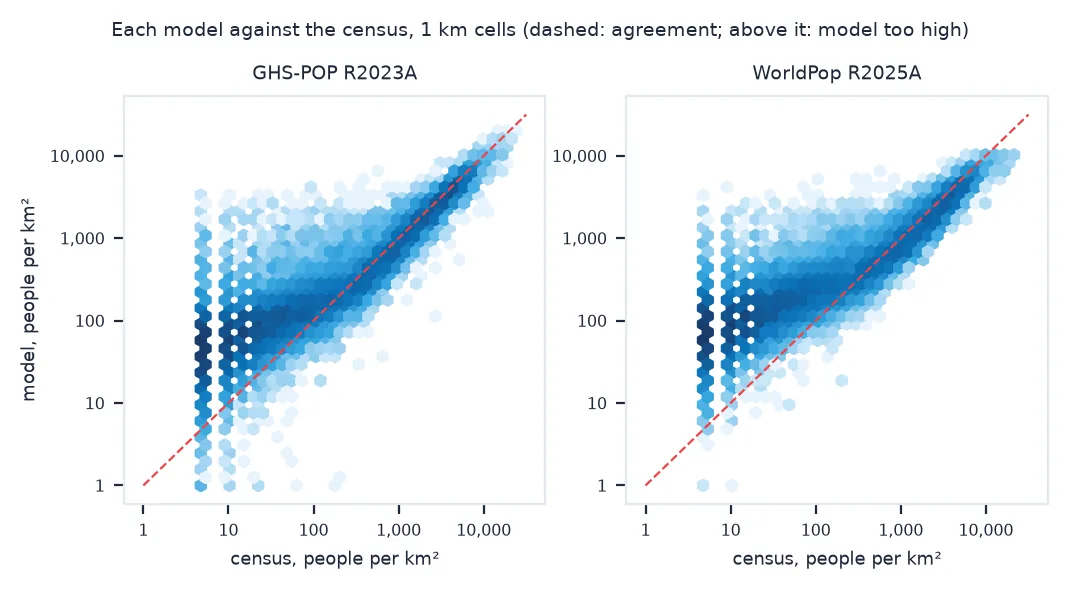
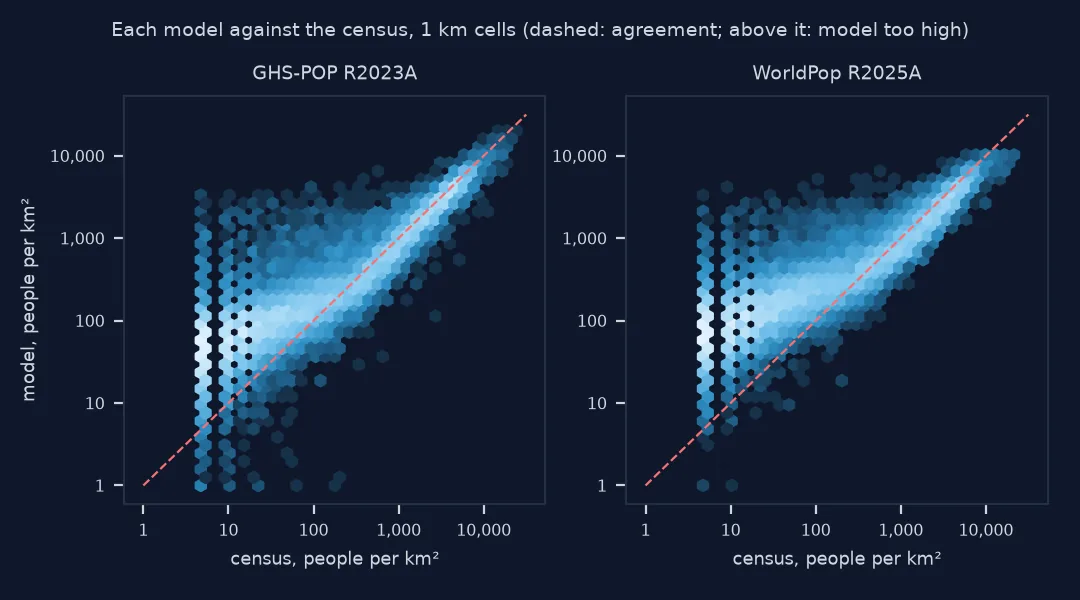
3. Errors by density
Group the cells by census density and look at the median error of each model in each group:
K["band"] = pd.cut(K.census, [0, 100, 500, 2_000, 5_000, 50_000], labels=["<100", "100-500", "500-2k", "2k-5k", "5k+"])
T = K.groupby("band", observed=True).apply(lambda g: pd.Series({
    "cells": len(g),
    "ghs_pop": f"{((g.ghs_pop - g.census) / g.census).median():+.0%}",
    "worldpop": f"{((g.worldpop - g.census) / g.census).median():+.0%}"}), include_groups=False)
print(T.to_string())
cells ghs_pop worldpop
band
<100 13663 +304% +530%
100-500 3932 +4% +43%
500-2k 3170 -15% -16%
2k-5k 2066 -13% -23%
5k+ 725 -15% -22%
The pattern is flattening. In cells with fewer than 100 residents, GHS-POP puts a median of four times as many people and WorldPop six times as many; in cells above 500 per km², both put 13% to 23% too few. The models spread people more evenly than the register shows they live.
Where GHS-POP disagrees most
The data used on this page
The CBS 100 m grid, final 2020 edition, GHS-POP R2023A epoch 2020 at 100 m in World Mollweide (tiles R3_C19 and R4_C19), and WorldPop R2025A constrained 2020 for the Netherlands; the land boundary from the PDOK CBS gebiedsindelingen web feature service limits the modelled grids to the country.
import io
import zipfile
from pathlib import Path

import geopandas as gpd
import numpy as np
import pandas as pd
import pyogrio
import rasterio
import requests
from pyproj import Transformer
from rasterio.features import geometry_mask
from rasterio.merge import merge

Path("data").mkdir(exist_ok=True)
GPKG = Path("data/cbs_vk100_2020_vol.gpkg")
if not GPKG.exists():
    url = "https://www.cbs.nl/-/media/cbs/dossiers/nederland-regionaal/vierkanten/100/2023-cbs_vk100_2020_vol.zip"
    zipfile.ZipFile(io.BytesIO(requests.get(url, timeout=900).content)).extract(GPKG.name, "data")
WP = Path("data/nld_pop_2020_CN_100m_R2025A_v1.tif")
if not WP.exists():
    WP.write_bytes(requests.get("https://data.worldpop.org/GIS/Population/Global_2015_2030/R2025A/2020/NLD/v1/100m/constrained/"
                                "nld_pop_2020_CN_100m_R2025A_v1.tif", timeout=600).content)
BASE = "https://jeodpp.jrc.ec.europa.eu/ftp/jrc-opendata/GHSL/GHS_POP_GLOBE_R2023A/GHS_POP_E2020_GLOBE_R2023A_54009_100/V1-0/tiles"
srcs = []
for t in ("R3_C19", "R4_C19"):
    tif = Path("data", f"GHS_POP_E2020_GLOBE_R2023A_54009_100_V1_0_{t}.tif")
    if not tif.exists():
        zipfile.ZipFile(io.BytesIO(requests.get(f"{BASE}/{tif.stem}.zip", timeout=900).content)).extract(tif.name, "data")
    srcs.append(rasterio.open(tif))
B = Path("data/landsdeel_2020.geojson")
if not B.exists():
    B.write_bytes(requests.get("https://service.pdok.nl/cbs/gebiedsindelingen/2020/wfs/v1_0", timeout=300, params={
        "service": "WFS", "version": "2.0.0", "request": "GetFeature", "typeName": "gebiedsindelingen:landsdeel_gegeneraliseerd",
        "outputFormat": "application/json", "srsName": "EPSG:28992"}).content)
NL = gpd.read_file(B).dissolve()
def cells(a, transform, crs):
    """Centres of the populated cells inside the Netherlands, in RD New metres, and their counts."""
    inside = ~geometry_mask(NL.to_crs(crs).geometry, a.shape, transform)
    r, c = np.nonzero(inside & (a > 0))
    x, y = rasterio.transform.xy(transform, r, c)
    X, Y = Transformer.from_crs(crs, 28992, always_xy=True).transform(np.asarray(x), np.asarray(y))
    return np.c_[X, Y], a[r, c].astype("float64")
g, gt = merge(srcs, bounds=(230_000, 5_930_000, 530_000, 6_280_000))
GHS_XY, GHS_POP = cells(g[0], gt, "ESRI:54009")
with rasterio.open(WP) as src:
    WP_XY, WP_POP = cells(src.read(1), src.transform, src.crs)
V = pyogrio.read_dataframe(GPKG, columns=["crs28992res100m", "aantal_inwoners"], read_geometry=False)
V = V[V.aantal_inwoners > 0]
CBS_XY = V.crs28992res100m.str.extract(r"E(\d+)N(\d+)").astype(int).to_numpy() * 100 + 50
CBS_POP = V.aantal_inwoners.to_numpy("float64")
def km(xy, pop):
    """Sum counts into 1 km RD New cells, indexed by the lower-left corner in km."""
    return pd.Series(pop).groupby([xy[:, 0] // 1000, xy[:, 1] // 1000]).sum()
print(f"census {CBS_POP.sum():,.0f}; GHS-POP inside the land boundary {GHS_POP.sum():,.0f}; WorldPop inside it {WP_POP.sum():,.0f}")
census 16,740,785; GHS-POP inside the land boundary 17,418,265; WorldPop inside it 17,589,165
Inside the land boundary, the census squares hold 16,740,785 residents, GHS-POP 17,418,265 and WorldPop 17,589,165.
Example 1: where GHS-POP disagrees most
List the 1 km cells with the largest differences in people, both ways, with their census count:
K["diff"] = K.ghs_pop - K.census
top = pd.concat([K.nlargest(3, "diff"), K.nsmallest(3, "diff")])
top.index = [f"x {a} km, y {b} km" for a, b in top.index]
print(top[["census", "ghs_pop", "worldpop", "diff"]].round(0).astype(int).to_string())
census ghs_pop worldpop diff
x 120.0 km, y 483.0 km 2815 8993 7695 6178
x 118.0 km, y 483.0 km 610 5969 6258 5359
x 124.0 km, y 480.0 km 345 5583 5307 5238
x 93.0 km, y 438.0 km 16135 6974 6410 -9161
x 91.0 km, y 438.0 km 16905 8050 7030 -8855
x 93.0 km, y 434.0 km 14455 6289 5208 -8166
GHS-POP's three largest overestimates are cells in the south of Amsterdam where the census registers 345 to 2,815 residents and both models put 5,300 to 9,000; its largest underestimates are three cells in Rotterdam with 14,455 to 16,905 registered residents, where both models put fewer than half. The two models make the same mistakes in the same cells, which points at what they share, the view from above, rather than at either model's details.
Counted residents against modelled spread
The census grid counts residents at their registered addresses; the models distribute municipal totals over cells using what can be seen from above. Where the two agree, the model's picture of residential building matches where people are registered; where they do not, the model has misjudged how residential a building is, how many people live in it, or has old inputs. GHS-POP's Dutch inputs are the 2011 register, carried forward; WorldPop's are not listed, but its municipal sums suggest later boundaries.
Census coverage and centre assignment
- Compare on cells the census covers: cells with no published census residents can hold real people below the publication threshold; restricting to cells with residents avoids scoring the models against suppression.
- Common grid choice: the comparison depends on the cell size; scores at 1 km do not carry over to 100 m or 5 km, so rerun it at the size the analysis uses.
- Assignment by centre: a fine cell's people go wholly into the 1 km cell containing its centre; with 100 m cells that shift is small, with 1 km sources it would not be.
- The census is not perfect either: it is rounded down to multiples of five and short by 667,000 people; differences of a few people per cell are within that noise.
Internal links
- How to sum a population grid by municipality in Python — the same models scored by area
- How to use a census population grid in Python — the reference grid
- How to resample a population grid to another resolution in Python — putting grids on a common grid
FAQ
How do I compare two population rasters in Python?
Put them on one grid by assigning each fine cell to a coarse cell by its centre and summing, then compare cell by cell: totals, the share of cells and people within a tolerance, and errors by density.
Which is more accurate, GHSL or WorldPop?
For the Netherlands in 2020, compared with the census at 1 km, GHS-POP gets 24% of cells within 25%, holding 60% of the people, and WorldPop R2025A 18% and 46%; results differ between countries and inputs.
Why do modelled population grids underestimate dense areas?
They distribute people by what satellites see, mostly built-up area and volume, which does not capture how many people live in each building, so they tend to spread people more evenly than they are.
Is correlation a good measure of population grid accuracy?
Not alone: it is high whenever cities and countryside are told apart. Report errors in people and the share of cells within a tolerance.