
How to Use a Census Population Grid in Python
On this page
Problem statement
Some statistical offices publish census or register counts on a regular grid, not just for administrative areas. Statistics Netherlands (CBS) publishes 100 m squares with residents by age and sex, households, dwellings and more, every year. A census grid is the closest thing to ground truth for gridded population: the counts come from addresses, not a model. It still needs care, because the values are rounded and partly suppressed for confidentiality, and the codes that mark suppression are numbers that sum.
This page reads the CBS 2020 100 m grid, handles the suppression code, turns the square IDs into a raster without reading the geometries, finds the densest squares, and aggregates the grid to 1 km to show what resolution does to density.
Quick answer
Read the attribute table only, treat negative values as missing, and sum:
cols = ["crs28992res100m", "aantal_inwoners", "aantal_inwoners_0_tot_15_jaar", "aantal_inwoners_65_jaar_en_ouder", "aantal_woningen"]
V = pyogrio.read_dataframe(GPKG, columns=cols, read_geometry=False)
pop = V.aantal_inwoners.where(V.aantal_inwoners >= 0)
print(f"{len(V):,} squares of 100 m; residents in published squares: {pop.sum():,.0f}")
print(f"squares with residents suppressed: {pop.isna().sum():,}; official population 1 January 2020: {OFFICIAL:,}")
383,061 squares of 100 m; residents in published squares: 16,740,785
squares with residents suppressed: 3,156; official population 1 January 2020: 17,407,585
The published squares hold 16,740,785 residents, 666,800 fewer than the official 17,407,585. 3,156 squares are published for their dwellings but have the resident count suppressed.
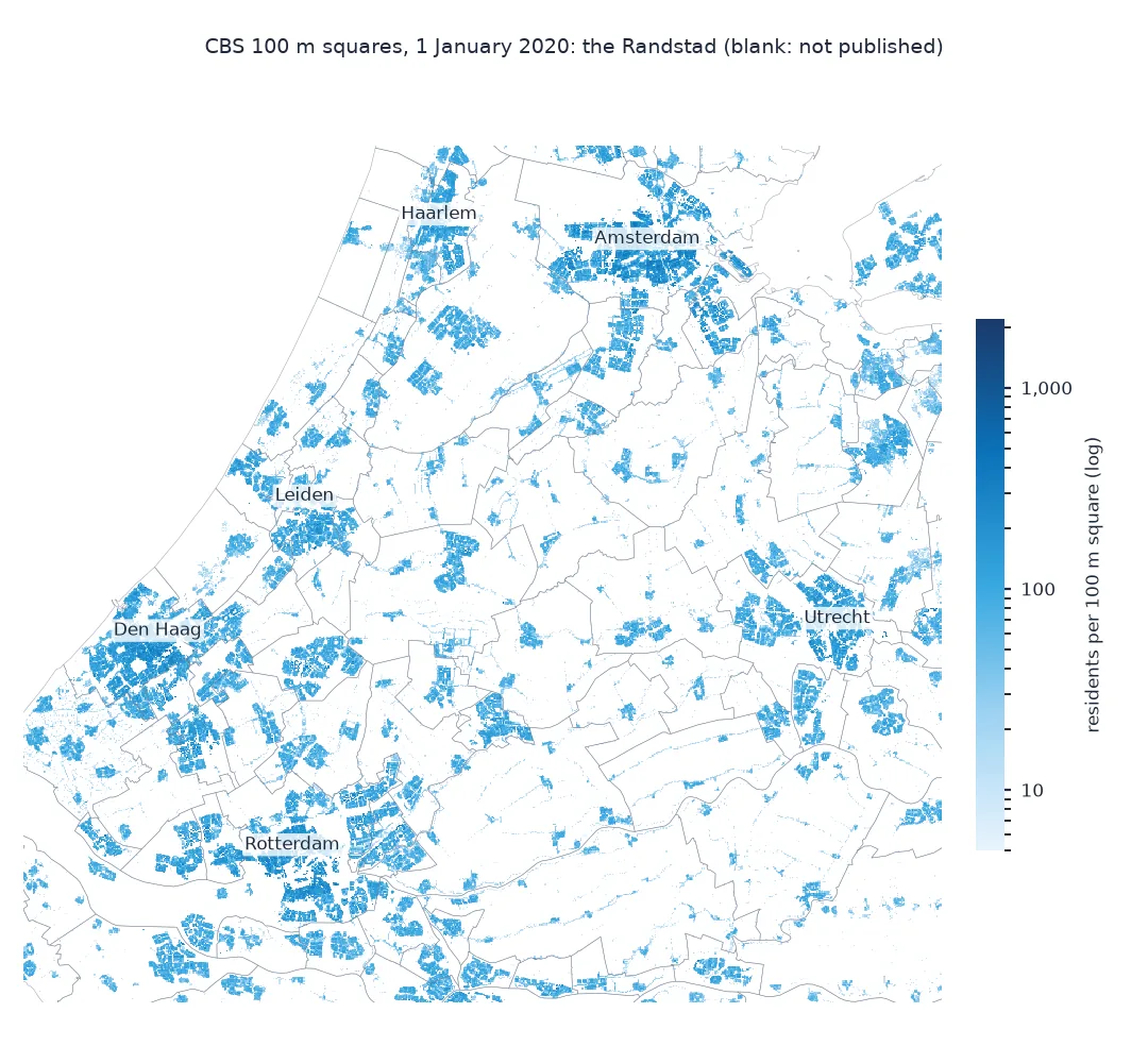
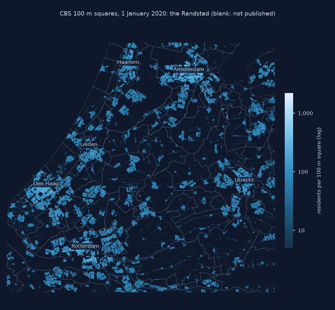
Recognise suppression, rasterise square ids, find the densest squares
1. Recognise the suppression code
CBS publishes a square only if it has at least five residents or five dwellings, rounds counts to multiples of five, and writes -99997 where a value is confidential. How often it does so differs by column:
for c in cols[1:]:
    v = V[c]
    print(f"{c:>34}: {(v == -99997).sum():>7,} suppressed, other negatives {((v < 0) & (v != -99997)).sum()}, "
          f"multiples of 5: {(v[v > 0] % 5 == 0).mean():.0%}")
naive = V.aantal_inwoners_0_tot_15_jaar.sum()
print(f"children under 15, summed without masking: {naive:,}")
aantal_inwoners: 3,156 suppressed, other negatives 0, multiples of 5: 100%
aantal_inwoners_0_tot_15_jaar: 206,592 suppressed, other negatives 0, multiples of 5: 100%
aantal_inwoners_65_jaar_en_ouder: 178,729 suppressed, other negatives 0, multiples of 5: 100%
aantal_woningen: 103,007 suppressed, other negatives 0, multiples of 5: 100%
children under 15, summed without masking: -20,656,260,619
Every value is a multiple of five, and -99997 is the only negative code. The resident count is suppressed in 3,156 squares, but the age bands in about 200,000, because a small band identifies people faster than a total. Summing the under-15 column as it stands gives minus 20.7 billion children.
2. Build a raster from the square IDs
The ID encodes each square's lower-left corner in hectometres in the Dutch RD New grid, EPSG:28992: E1748N3174 is the square from x 174,800 m, y 317,400 m. Parsing it is faster than reading 383,061 polygons:
xy = V.crs28992res100m.str.extract(r"E(\d+)N(\d+)").astype(int)
x0, y1 = xy[0].min(), xy[1].max() + 1
R = np.zeros((y1 - xy[1].min(), xy[0].max() + 1 - x0), dtype="float32")
R[y1 - 1 - xy[1], xy[0] - x0] = pop.fillna(0).to_numpy()
transform = rasterio.transform.from_origin(x0 * 100, y1 * 100, 100, 100)
print(f"raster {R.shape[1]} x {R.shape[0]} cells of 100 m; total {R.sum(dtype='float64'):,.0f}; origin {x0 * 100:,} E, {y1 * 100:,} N")
raster 2636 x 3040 cells of 100 m; total 16,740,785; origin 13,900 E, 611,500 N
The raster is 2,636 by 3,040 cells with its top-left corner at x 13,900 m, y 611,500 m, and holds the same 16,740,785 residents as the table: no square was lost or doubled.
3. The densest squares and where they are
Join the densest squares to the municipality boundaries by their centres:
top = V.assign(x=xy[0] * 100 + 50, y=xy[1] * 100 + 50, pop=pop).nlargest(5, "pop")
pts = gpd.GeoDataFrame(top, geometry=gpd.points_from_xy(top.x, top.y), crs=28992).sjoin(GM[["statnaam", "geometry"]])
print(pts[["crs28992res100m", "pop", "aantal_woningen", "statnaam"]].to_string(index=False))
crs28992res100m pop aantal_woningen statnaam
E1748N3174 2180.0 -99997 Maastricht
E1179N4872 2055.0 -99997 Amsterdam
E0828N4540 1820.0 -99997 's-Gravenhage
E0930N4374 1410.0 125 Rotterdam
E2660N5453 1150.0 -99997 Westerwolde
The five densest squares are in Maastricht, Amsterdam, Den Haag, Rotterdam and Westerwolde, with 1,150 to 2,180 residents each. Four of them have their dwelling count suppressed: over a thousand residents at a handful of addresses, which most likely means communal establishments such as student housing, care homes or a reception centre rather than ordinary flats. Only the Rotterdam square shows 125 dwellings.
The same people at 1 km
The data used on this page
The CBS Kaart van 100 meter bij 100 meter met statistieken, final 2020 edition (residents on 1 January 2020), the 2020 municipality boundaries from the PDOK CBS gebiedsindelingen web feature service, and the population on 1 January 2020 from StatLine table 03759ned.
import io
import json
import zipfile
from pathlib import Path

import geopandas as gpd
import numpy as np
import pyogrio
import rasterio
import requests

Path("data").mkdir(exist_ok=True)
GPKG = Path("data/cbs_vk100_2020_vol.gpkg")
if not GPKG.exists():
    url = "https://www.cbs.nl/-/media/cbs/dossiers/nederland-regionaal/vierkanten/100/2023-cbs_vk100_2020_vol.zip"
    zipfile.ZipFile(io.BytesIO(requests.get(url, timeout=900).content)).extract(GPKG.name, "data")
B = Path("data/gemeente_2020.geojson")
if not B.exists():
    B.write_bytes(requests.get("https://service.pdok.nl/cbs/gebiedsindelingen/2020/wfs/v1_0", timeout=300, params={
        "service": "WFS", "version": "2.0.0", "request": "GetFeature", "typeName": "gebiedsindelingen:gemeente_gegeneraliseerd",
        "outputFormat": "application/json", "srsName": "EPSG:28992"}).content)
GM = gpd.read_file(B)
C = Path("data/cbs_pop_2020.json")
if not C.exists():
    C.write_bytes(requests.get("https://opendata.cbs.nl/ODataApi/odata/03759ned/TypedDataSet", timeout=300, params={
        "$filter": "Geslacht eq 'T001038' and Leeftijd eq '10000' and BurgerlijkeStaat eq 'T001019' and Perioden eq '2020JJ00' "
                   "and (substring(RegioS,0,2) eq 'GM' or substring(RegioS,0,2) eq 'NL')",
        "$select": "RegioS,BevolkingOp1Januari_1"}).content)
OFFICIAL = next(r["BevolkingOp1Januari_1"] for r in json.loads(C.read_text())["value"] if r["RegioS"].startswith("NL"))
info = pyogrio.read_info(GPKG)
print(f"{GPKG.name}: {GPKG.stat().st_size / 1e6:,.0f} MB, {info['features']:,} squares, {len(info['fields'])} columns, {info['crs']}; {len(GM)} municipalities")
cbs_vk100_2020_vol.gpkg: 639 MB, 383,061 squares, 129 columns, EPSG:28992; 355 municipalities
The GeoPackage is 639 MB with 383,061 squares and 129 columns in EPSG:28992; reading five columns without geometry takes seconds.
Example 1: the same people at 1 km
Sum the 100 m squares into 1 km squares by integer division of the IDs, and compare the densest square at each resolution, both as people per km²:
km = V.assign(kx=xy[0] // 10, ky=xy[1] // 10, pop=pop.fillna(0)).groupby(["kx", "ky"]).pop.sum()
print(f"1 km squares with residents: {(km > 0).sum():,}; total {km.sum():,.0f}")
print(f"densest 100 m square: {pop.max() * 100:,.0f} people per km2; densest 1 km square: {km.max():,.0f} per km2")
print(f"people in 1 km squares above 10,000 per km2: {km[km > 10_000].sum():,.0f}; in 100 m squares above the same density: {pop[pop > 100].sum():,.0f}")
1 km squares with residents: 23,556; total 16,740,785
densest 100 m square: 218,000 people per km2; densest 1 km square: 23,165 per km2
people in 1 km squares above 10,000 per km2: 1,107,155; in 100 m squares above the same density: 4,712,315
Aggregated to 23,556 squares of 1 km, the total is unchanged but the peaks flatten: the densest 100 m square is 218,000 people per km², the densest 1 km square 23,165. At 1 km, 1.1 million people live in squares above 10,000 per km²; at 100 m, 4.7 million live in squares that dense. Density is a property of the grid as much as of the place.
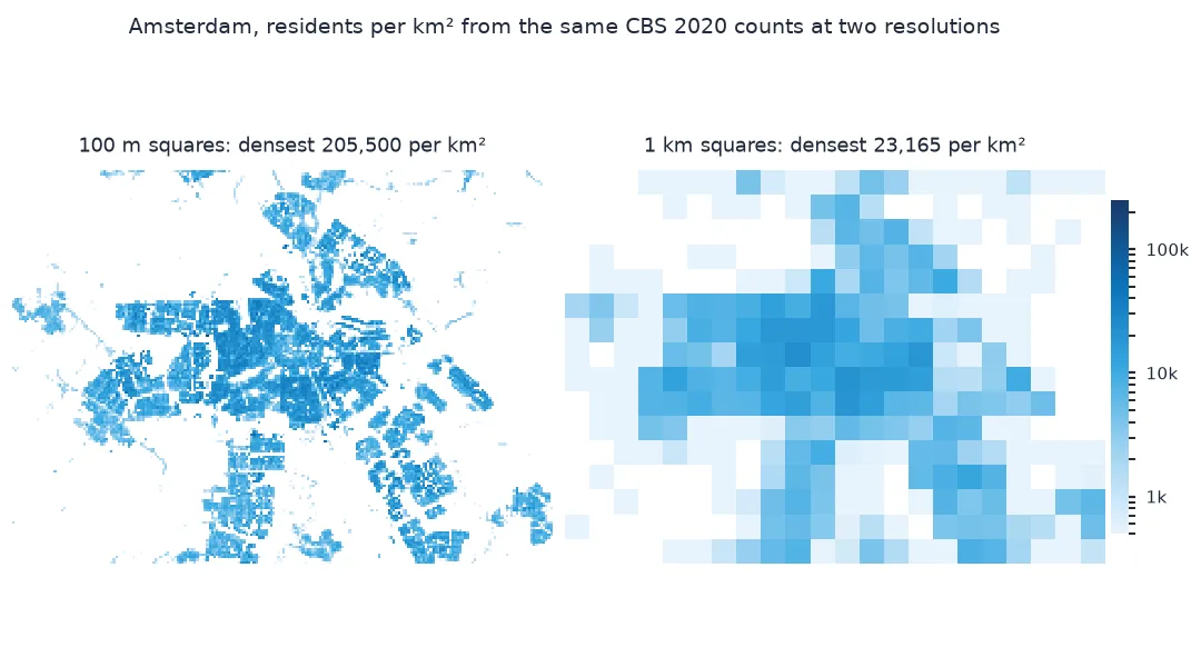
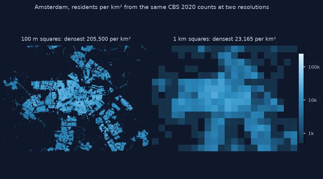
A census grid is built bottom up
A census grid is built bottom up. CBS geocodes every registered resident to the address where they live, using the population register (BRP) and the national address and buildings register (BAG), and counts the addresses that fall in each square. No model distributes anyone: a square has the people whose homes are in it. That is why a census grid is the yardstick for modelled grids such as GHS-POP and WorldPop.
The price of that precision is confidentiality. A 100 m square can contain a single household, so CBS drops squares with fewer than five residents and five dwellings, rounds what it publishes to multiples of five, and suppresses any value that could identify someone. The suppression code is written into the numeric column, so a careless sum subtracts 99,997 for every suppressed square. And the published squares do not add up to the official total: every municipality comes out short, which the census grid total page works through.
Changing columns and stricter rules
- Columns change by year: field names and categories differ between editions; check
pyogrio.read_infobefore reusing code on another year. - Provisional and final: CBS publishes a provisional edition (
v1) and later a final one (vol); the counts can change between them. - Stricter rules from 2025: CBS tightened its confidentiality rules for the 2025 reporting year, so later editions publish less than earlier ones.
- Other countries: Eurostat's 1 km census grids for 2011 and 2021 cover the whole EU with one schema, at coarser resolution.
Internal links
- How to download and clip the GHSL population grid in Python — a modelled grid for comparison
- How to suppress small counts in Python — the publisher's side of suppression
- How to download and use a WorldPop population raster in Python — another modelled grid
FAQ
How do I read the CBS 100 m grid in Python?
Download the zipped GeoPackage from the CBS website and read it with pyogrio.read_dataframe; pass read_geometry=False and columns= when only the counts are needed, and parse the square ID for coordinates.
What does -99997 mean in CBS grid data?
It marks a suppressed value. Replace it with a missing value before summing or averaging.
Why does the CBS grid total not match the population of the Netherlands?
Squares with fewer than five residents and five dwellings are not published, and published counts are rounded; together they leave the 2020 grid about 667,000 people short of the official count.
How do I convert a CBS square ID to coordinates?
E1748N3174 means the lower-left corner is at x 174,800 m and y 317,400 m in EPSG:28992; multiply the two numbers by 100.