How to Resample a Population Grid to Another Resolution in Python

Problem statement

Population grids rarely arrive at the resolution or on the grid an analysis needs. A 100 m grid is too fine to map a country, a square grid has to become hexagons for a dashboard, and a national census grid has to be put on the European reference grid to be combined with other countries. Each of these is an aggregation of counts, and done right it keeps every person exactly once. Done with a generic resampling method it loses or invents people, as the reprojection fix shows.

This page aggregates GHS-POP from 100 m to 1 km by block summing and checks the result against the 1 km product the JRC publishes, sums Statistics Netherlands' 100 m census squares into H3 hexagons, and moves them onto the EU's 1 km reference grid in EPSG:3035.

Quick answer

When the coarse cells are whole blocks of fine ones on the same grid, reshape and sum; nothing is interpolated:

f = 10                                                                    # 10 x 10 cells of 100 m = 1 km
h, w = (P100.shape[0] // f) * f, (P100.shape[1] // f) * f
P1k = P100[:h, :w].reshape(h // f, f, w // f, f).sum(axis=(1, 3))
print(f"100 m: {P100.shape[1]} x {P100.shape[0]} cells, {P100.sum():,.0f} people")
print(f"1 km:  {P1k.shape[1]} x {P1k.shape[0]} cells, {P1k.sum():,.0f} people")

100 m: 3000 x 3500 cells, 36,568,535 people
1 km:  300 x 350 cells, 36,568,535 people

The window, a rectangle around the Netherlands that also takes in parts of Belgium and Germany, holds 36,568,535 people in 3,000 by 3,500 cells of 100 m, and exactly the same number in 300 by 350 cells of 1 km.

Line blocks up, compare with the 1 km product, hexagons

1. Line the blocks up with the coarse grid

Block summing is only exact if the fine grid's origin falls on a coarse cell corner. GHS-POP's 100 m and 1 km Mollweide tiles share their corners, so read a window whose bounds are whole kilometres:

print(f"window: x {BOUNDS[0]:,.0f} to {BOUNDS[2]:,.0f}, y {BOUNDS[1]:,.0f} to {BOUNDS[3]:,.0f} m (whole km: {all(b % 1000 == 0 for b in BOUNDS)})")
print(f"100 m origin {T100.c:,.0f}, {T100.f:,.0f}; 1 km origin {T1K.c:,.0f}, {T1K.f:,.0f}")

window: x 230,000 to 530,000, y 5,930,000 to 6,280,000 m (whole km: True)
100 m origin 230,000, 6,280,000; 1 km origin 230,000, 6,280,000

Both windows start at x 230,000 m and y 6,280,000 m, a whole-kilometre corner, so every 1 km cell is exactly ten by ten 100 m cells.

2. Compare with the published 1 km product

The JRC publishes GHS-POP at 1 km as a separate product. If it is the 100 m grid summed, the two match cell for cell:

d = P1k - G1K
print(f"published 1 km: {G1K.sum():,.0f} people; block sum: {P1k.sum():,.0f}")
print(f"cells: {d.size:,}; identical to 1 person: {(np.abs(d) < 1).mean():.1%}; largest difference {np.abs(d).max():,.0f}")
print(f"correlation {np.corrcoef(P1k.ravel(), G1K.ravel())[0, 1]:.4f}")

published 1 km: 36,568,535 people; block sum: 36,568,535
cells: 105,000; identical to 1 person: 100.0%; largest difference 0
correlation 1.0000

The block sum and the published 1 km product are identical: all 105,000 cells agree to within one person, with a largest difference of zero. GHS-POP's 1 km Mollweide grid is its 100 m grid aggregated, so either can be derived from the other.

3. Squares into hexagons

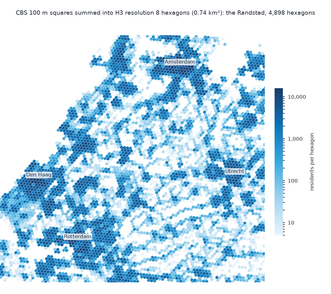
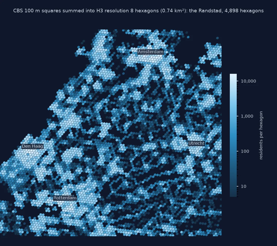
H3 cells do not nest with squares, so assign each 100 m square to the hexagon containing its centre and sum. At resolution 8 a hexagon averages 0.74 km², about 74 squares:

lon, lat = Transformer.from_crs(28992, 4326, always_xy=True).transform(SQ.x * 100 + 50, SQ.y * 100 + 50)
SQ["h3"] = [h3.latlng_to_cell(b, a, 8) for a, b in zip(lon, lat)]
H = SQ.groupby("h3").residents.sum()
print(f"{len(SQ):,} squares into {len(H):,} hexagons; total {H.sum():,} = {SQ.residents.sum():,}")
print(f"squares per hexagon: median {SQ.groupby('h3').size().median():.0f}; most residents in one hexagon {H.max():,}")

379,905 squares into 32,222 hexagons; total 16,740,785 = 16,740,785
squares per hexagon: median 4; most residents in one hexagon 15,560

The 379,905 squares fall into 32,222 hexagons, and the total is unchanged at 16,740,785. A median hexagon holds only 4 populated squares, because most hexagons cover sparsely settled land; the fullest holds 15,560 residents.

Onto the EU reference grid

The data used on this page

GHS-POP R2023A epoch 2020 in World Mollweide at 100 m and at 1 km (tiles R3_C19 and R4_C19), and the CBS 100 m grid, final 2020 edition.

import io
import zipfile
from pathlib import Path

import h3
import numpy as np
import pyogrio
import rasterio
import requests
from pyproj import Transformer
from rasterio.merge import merge

Path("data").mkdir(exist_ok=True)
BASE = "https://jeodpp.jrc.ec.europa.eu/ftp/jrc-opendata/GHSL/GHS_POP_GLOBE_R2023A"
def tiles(res):
    out = []
    for t in ("R3_C19", "R4_C19"):
        tif = Path("data", f"GHS_POP_E2020_GLOBE_R2023A_54009_{res}_V1_0_{t}.tif")
        if not tif.exists():
            url = f"{BASE}/GHS_POP_E2020_GLOBE_R2023A_54009_{res}/V1-0/tiles/{tif.stem}.zip"
            zipfile.ZipFile(io.BytesIO(requests.get(url, timeout=900).content)).extract(tif.name, "data")
        out.append(rasterio.open(tif))
    return out
BOUNDS = (230_000, 5_930_000, 530_000, 6_280_000)                         # the Netherlands in Mollweide, whole km
a100, T100 = merge(tiles(100), bounds=BOUNDS)
a1k, T1K = merge(tiles(1000), bounds=BOUNDS)
P100, G1K = np.where(a100[0] > 0, a100[0], 0).astype("float64"), np.where(a1k[0] > 0, a1k[0], 0).astype("float64")
GPKG = Path("data/cbs_vk100_2020_vol.gpkg")
if not GPKG.exists():
    url = "https://www.cbs.nl/-/media/cbs/dossiers/nederland-regionaal/vierkanten/100/2023-cbs_vk100_2020_vol.zip"
    zipfile.ZipFile(io.BytesIO(requests.get(url, timeout=900).content)).extract(GPKG.name, "data")
V = pyogrio.read_dataframe(GPKG, columns=["crs28992res100m", "aantal_inwoners"], read_geometry=False)
SQ = V[V.aantal_inwoners > 0].copy()
SQ[["x", "y"]] = SQ.crs28992res100m.str.extract(r"E(\d+)N(\d+)").astype(int).to_numpy()
SQ["residents"] = SQ.aantal_inwoners
print(f"GHS-POP 100 m window {P100.shape}, 1 km window {G1K.shape}; CBS squares with residents: {len(SQ):,}")

GHS-POP 100 m window (3500, 3000), 1 km window (350, 300); CBS squares with residents: 379,905

The merged windows are 3,500 by 3,000 cells at 100 m and 350 by 300 at 1 km; 379,905 CBS squares have a published resident count.

Example 1: onto the EU 1 km reference grid

The European statistical grid is 1 km squares in EPSG:3035, named by their lower-left corner in kilometres. Reproject each square's centre, floor to the kilometre, and sum:

x, y = Transformer.from_crs(28992, 3035, always_xy=True).transform(SQ.x * 100 + 50, SQ.y * 100 + 50)
SQ["eu1km"] = ["1kmN%dE%d" % (b // 1000, a // 1000) for a, b in zip(x, y)]
E = SQ.groupby("eu1km").residents.sum()
print(f"{len(E):,} EU 1 km cells with residents; total {E.sum():,}")
print(f"densest: {E.idxmax()} with {E.max():,}; squares per EU cell: median {SQ.groupby('eu1km').size().median():.0f}")

23,842 EU 1 km cells with residents; total 16,740,785
densest: 1kmN3261E3973 with 24,590; squares per EU cell: median 6

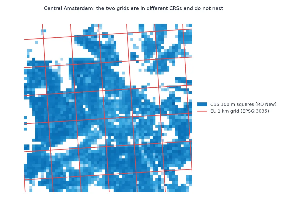
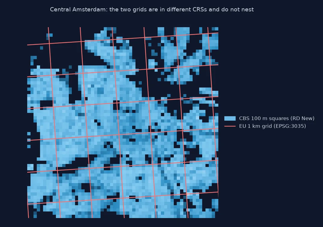
On the EU 1 km grid the squares make 23,842 populated cells, again 16,740,785 people in all. The fullest, 1kmN3261E3973, holds 24,590 residents; a median EU cell gets 6 CBS squares, because the many sparsely settled cells have few populated squares.

When aggregation keeps the total exactly

Aggregation keeps a population total exactly when every fine cell is assigned to one coarse cell and its count is added there. Block summing on nested grids does that by construction. Assigning by centre does it for grids that do not nest, such as squares into hexagons or one national grid onto another, at the cost of moving each fine cell's people to wherever its centre falls; with 100 m squares going into cells of 0.7 to 1 km², that shift is small next to the cell size.

The comparison with the published 1 km product shows what a consistent product family looks like: GHS-POP's 1 km Mollweide grid is its 100 m grid summed, to the person, so the two can be mixed freely. That is worth checking rather than assuming for any pair of products; when one is not the aggregate of the other, derive the coarse one from the fine one yourself, so the numbers at both scales agree.

Nearly nesting grids and suppressed squares

• Grids that nearly nest: the CBS 100 m squares and the RD New 1 km grid nest; the CBS squares and the EU 1 km grid do not, because they are in different CRSs, so they need centre assignment.
• Edges of a block sum: a window that is not a whole number of blocks leaves partial blocks; crop to whole kilometres first, as here, or pad with zeros.
• Hexagon resolution: H3 resolutions step by a factor of about 7 in area; resolution 7 averages 5.2 km² and resolution 9 0.11 km², close to a 100 m square, too fine to aggregate into.
• Suppressed squares stay missing: aggregating the CBS grid does not recover suppressed or unpublished squares; the totals keep their shortfall.

Internal links

• Fixing a population total that changes after reprojecting the grid — what goes wrong with interpolation
• How to use a census population grid in Python — the CBS squares
• How to download and clip the GHSL population grid in Python — the GHSL product family

FAQ

How do I aggregate a population raster to a coarser resolution in Python?

If the coarse grid nests in the fine one, reshape the array into blocks and sum: a.reshape(h // f, f, w // f, f).sum(axis=(1, 3)). Otherwise assign each fine cell to a coarse cell by its centre and sum with groupby.

Is GHSL 1 km the same as GHSL 100 m summed?

For the Mollweide grids, yes: over the Netherlands and its neighbours the R2023A 1 km product equals the 100 m product summed in 10 by 10 blocks, cell for cell.

How do I put population on H3 hexagons?

Convert each cell centre to latitude and longitude, get its H3 cell with h3.latlng_to_cell, and sum by hexagon.

What is the EU 1 km grid?

The European statistical reference grid of 1 km squares in EPSG:3035, named by the lower-left corner, for example 1kmN3200E4000.