Fixing a Population Total That Changes After Reprojecting the Grid

Problem statement

A population grid in latitude and longitude is reprojected to a national grid so it lines up with other layers, and the country's population changes: millions too many, or a few percent too few, depending on the target cell size and the resampling method. The cause is that a population grid stores counts per cell, and every standard resampling method treats values as if they were densities or categories. A count copied by nearest neighbour into a cell twice as big counts its people once where there should be the sum of two cells; interpolated bilinearly into a cell half as big, it counts them twice.

This page reprojects GHS-POP 2020 from 30 arc-seconds to the Dutch RD New grid at 1 km and at 100 m with each common method, measures the error in the total, and fixes it two ways: resampling with sum, and converting to density before resampling and back to counts afterwards.

Quick answer

Never warp counts with nearest, bilinear or average. Warp a density with average and multiply by the new cell area, or use Resampling.sum:

dens = pop / cell_km2                                                    # people per km2 on the source grid
out = warp(dens, Resampling.average, 1000) * 1.0                         # 1 km cells: 1 km2 each
for label, total in (("source grid", pop.sum()),
                     ("counts, nearest", warp(pop, Resampling.nearest, 1000).sum()),
                     ("counts, bilinear", warp(pop, Resampling.bilinear, 1000).sum()),
                     ("density, average, x area", out.sum())):
    print(f"{label:>26}: {total:>12,.0f}  ({total / pop.sum() - 1:+.2%})")

               source grid:   17,389,161  (+0.00%)
           counts, nearest:    9,157,658  (-47.34%)
          counts, bilinear:    9,210,596  (-47.03%)
  density, average, x area:   17,386,586  (-0.01%)

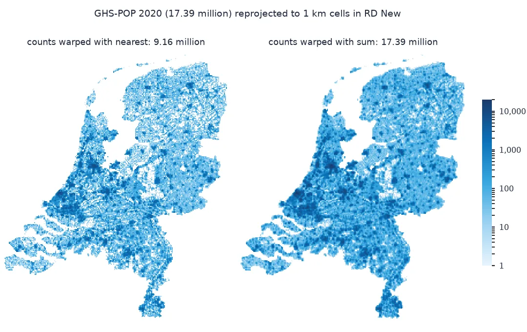
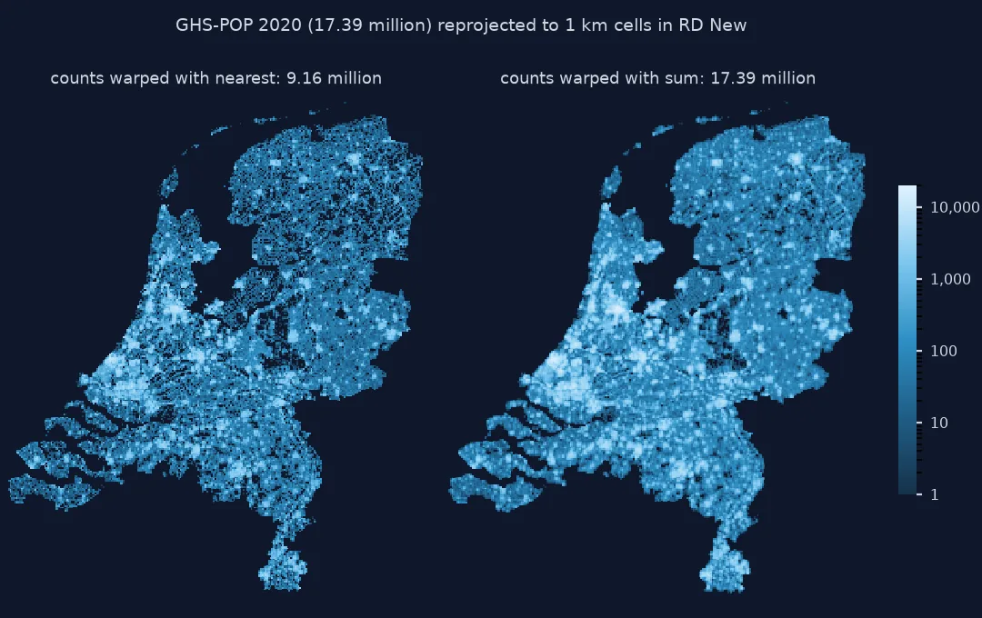
Warped to 1 km cells by nearest neighbour, the Netherlands loses 47% of its people: 9.2 million instead of 17.4 million. Bilinear does no better. Converting to density, averaging, and multiplying by the 1 km² of each new cell keeps the total within 0.01%.

Every method at two sizes, counts against densities, the fix

1. Every method at two target sizes

The error depends on the ratio of the target cell area to the source cell area. A 30 arc-second cell in the Netherlands is about 0.53 km², so a 1 km cell is about twice as big and a 100 m cell about 53 times smaller:

methods = ["nearest", "bilinear", "cubic", "average", "sum"]
for size in (1000, 100):
    row = {m: warp(pop, getattr(Resampling, m), size).sum() / pop.sum() - 1 for m in methods}
    print(f"{size:>5} m: " + "  ".join(f"{m} {v:+.1%}" for m, v in row.items()))

 1000 m: nearest -47.3%  bilinear -47.0%  cubic -47.0%  average -47.1%  sum +0.0%
  100 m: nearest +5198.1%  bilinear +5194.6%  cubic +5194.9%  average +5194.7%  sum +0.0%

At 1 km every method that treats the values as point samples, including average, loses about 47%; at 100 m they multiply the population 53 times, to over 900 million. Only sum keeps the total at both sizes.

2. Why counts and densities behave differently

At 1 km, nearest neighbour gives each target cell the count of the one source cell under its centre. Compare the target cell's area with the source cell's to see the factor that error follows:

src_mean = cell_km2[~pop.mask].mean()
print(f"mean source cell area: {src_mean:.3f} km2; 1 km target: {1 / src_mean:.2f} source cells per target cell")
print(f"nearest at 1 km undercounts by about 1 - {src_mean:.3f}: expected {src_mean - 1:+.1%}")
print(f"at 100 m each source cell is copied into about {src_mean / 0.01:.0f} target cells")

mean source cell area: 0.528 km2; 1 km target: 1.89 source cells per target cell
nearest at 1 km undercounts by about 1 - 0.528: expected -47.2%
at 100 m each source cell is copied into about 53 target cells

A source cell covers 0.528 km² on average, so a 1 km cell spans 1.89 of them. Nearest neighbour keeps one, so the expected loss is 1 minus 0.528, -47.2%, exactly what step 1 found. At 100 m each source count lands in about 53 target cells.

3. The density fix at 100 m

In the GDAL used here, sum also kept the total at 100 m, so it weights each source cell by the share of it inside each target cell. The density route does not depend on that: convert to density, warp with any interpolating method, and multiply by the target cell area:

for m in ("nearest", "bilinear", "average"):
    t = (warp(dens, getattr(Resampling, m), 100) * 0.01).sum()
    print(f"density, {m:>8}, x 0.01 km2: {t:,.0f}  ({t / pop.sum() - 1:+.2%})")

density,  nearest, x 0.01 km2: 17,397,483  (+0.05%)
density, bilinear, x 0.01 km2: 17,385,794  (-0.02%)
density,  average, x 0.01 km2: 17,386,060  (-0.02%)

Through density, all three methods keep the total within 0.05% at 100 m, even nearest neighbour, because a density copied into a smaller cell is still the right density there.

Checking cell by cell, not just the total

The data used on this page

GHS-POP R2023A epoch 2020 at 30 arc-seconds (tile R4_C19), clipped to the 2020 country boundary from the PDOK CBS gebiedsindelingen web feature service. The target grids are RD New (EPSG:28992) at 1 km and 100 m, aligned to whole kilometres.

import io
import zipfile
from pathlib import Path

import geopandas as gpd
import numpy as np
import rasterio
import requests
from pyproj import Geod
from rasterio.mask import mask
from rasterio.transform import from_origin
from rasterio.warp import Resampling, reproject

Path("data").mkdir(exist_ok=True)
name = "GHS_POP_E2020_GLOBE_R2023A_4326_30ss"
GHS = Path("data", f"{name}_V1_0_R4_C19.tif")
if not GHS.exists():
    url = f"https://jeodpp.jrc.ec.europa.eu/ftp/jrc-opendata/GHSL/GHS_POP_GLOBE_R2023A/{name}/V1-0/tiles/{GHS.stem}.zip"
    zipfile.ZipFile(io.BytesIO(requests.get(url, timeout=600).content)).extract(GHS.name, "data")
B = Path("data/landsdeel_2020.geojson")
if not B.exists():
    B.write_bytes(requests.get("https://service.pdok.nl/cbs/gebiedsindelingen/2020/wfs/v1_0", timeout=300, params={
        "service": "WFS", "version": "2.0.0", "request": "GetFeature", "typeName": "gebiedsindelingen:landsdeel_gegeneraliseerd",
        "outputFormat": "application/json", "srsName": "EPSG:28992"}).content)
NL = gpd.read_file(B).dissolve()
with rasterio.open(GHS) as src:
    a, tf = mask(src, NL.to_crs(src.crs).geometry, crop=True, filled=False)
    crs = src.crs
pop = a[0]
geod = Geod(ellps="WGS84")
row_km2 = np.array([abs(geod.polygon_area_perimeter([0, tf.a, tf.a, 0], [la, la, la + tf.e, la + tf.e])[0]) / 1e6
                    for la in tf.f + tf.e * np.arange(pop.shape[0])])
cell_km2 = np.broadcast_to(row_km2[:, None], pop.shape)
x0, y0, x1, y1 = (np.array(NL.total_bounds) // 1000 * 1000 + [0, 0, 1000, 1000])
def warp(values, method, size):
    """Reproject a masked source array onto an RD New grid of `size` metres."""
    out = np.zeros((int((y1 - y0) // size), int((x1 - x0) // size)), dtype="float64")
    reproject(values.filled(0).astype("float64"), out, src_transform=tf, src_crs=crs, dst_transform=from_origin(x0, y1, size, size),
              dst_crs="EPSG:28992", resampling=method, src_nodata=None, dst_nodata=None)
    return out
print(f"GDAL {rasterio.__gdal_version__}; source: {pop.count():,} cells, {pop.sum():,.0f} people; target extent {(x1 - x0) / 1000:.0f} x {(y1 - y0) / 1000:.0f} km")

GDAL 3.12.4; source: 66,493 cells, 17,389,161 people; target extent 266 x 314 km

The run uses GDAL 3.12.4. The source has 66,493 cells and 17,389,161 people; the target grid covers 266 by 314 km.

Example 1: check the result cell by cell, not only the total

A correct total can hide a smeared pattern. Compare the 1 km result of each correct method with the source's densest cell:

s = warp(pop, Resampling.sum, 1000)
d = warp(dens, Resampling.average, 1000)
print(f"source densest cell: {(pop / cell_km2).max():,.0f} per km2")
print(f"1 km, sum:              total {s.sum():,.0f}, densest {s.max():,.0f} per km2")
print(f"1 km, density average:  total {d.sum():,.0f}, densest {d.max():,.0f} per km2")
print(f"cells where the two differ by more than 1%: {(np.abs(s - d) > 0.01 * np.maximum(s, 1)).sum():,} of {(s > 0).sum():,}")

source densest cell: 21,534 per km2
1 km, sum:              total 17,389,161, densest 17,478 per km2
1 km, density average:  total 17,386,586, densest 17,495 per km2
cells where the two differ by more than 1%: 18,474 of 36,210

Both correct methods flatten the densest cell from 21,534 to about 17,500 per km², because a 1 km cell mixes it with its neighbours, and both keep the total. They are not identical cell by cell: half the populated cells differ by more than 1%, because the two methods share out boundary cells differently. Neither is wrong; pick one and use it throughout.

Resampling answers what is at a location

Resampling methods answer the question "what is the value at this location?" For a temperature, a density or an elevation, the value at a location is meaningful and interpolating it is right. For a count, the value belongs to the area of the cell, not to a location: 500 people in a cell of 0.53 km² are 500 people of that cell. Copying the count into a 1 km cell, as nearest neighbour does, drops the people of the source cells whose centres were not chosen; spreading it into 53 cells of 100 m, as nearest and bilinear do, multiplies them.

Densities can be resampled, because they are intensive: people per km² at a location does not depend on the size of the cell it is stored in. So the safe sequence is counts to density, using each source cell's true area, resample the density, and density back to counts, using each target cell's area. Resampling.sum, available in GDAL 3.1 and later, does the bookkeeping directly; in the GDAL version used here it kept the total at both target sizes.

GDAL sum support, nodata and snapping

• Check sum on your GDAL: here it preserved the total for coarser and finer targets alike; on an older GDAL, test it on a known total before relying on it for finer targets.
• Nodata: masked cells must be filled with zero before warping; otherwise the edges of the country lose people to nodata, or average ignores them and inflates edge cells.
• Area of the source cells: on a latitude-longitude grid each row has its own area; using one constant puts the error back in.
• Snap the target grid: align the target to whole kilometres, or to the grid of the layer it must match; an arbitrary origin shifts every cell boundary.

Internal links

• How to resample a population grid to another resolution in Python — aggregation done deliberately
• Fixing population densities that are wrong on latitude-longitude grids — the source cell areas
• How to download and clip the GHSL population grid in Python — the source grid

FAQ

Why did my population total change after reprojecting?

The grid holds counts, and nearest, bilinear and cubic resampling treat them as values at a point; each target cell gets a count meant for a different area. Resample densities, or use Resampling.sum for coarser targets.

What resampling method should I use for population?

sum, after checking that it preserves a known total on your GDAL; or convert to density, resample with average or bilinear, and multiply by the target cell area.

Does average resampling preserve population?

Only if applied to densities: averaging counts gives each larger cell the mean count of the small cells, not their sum.

How do I check a reprojected population grid?

Compare the totals before and after, and then the pattern: the densest cell, and a few areas summed in both grids.