Radar Rainfall Map Has Spokes and Hot Spots: Beam Blockage and Clutter

Problem statement

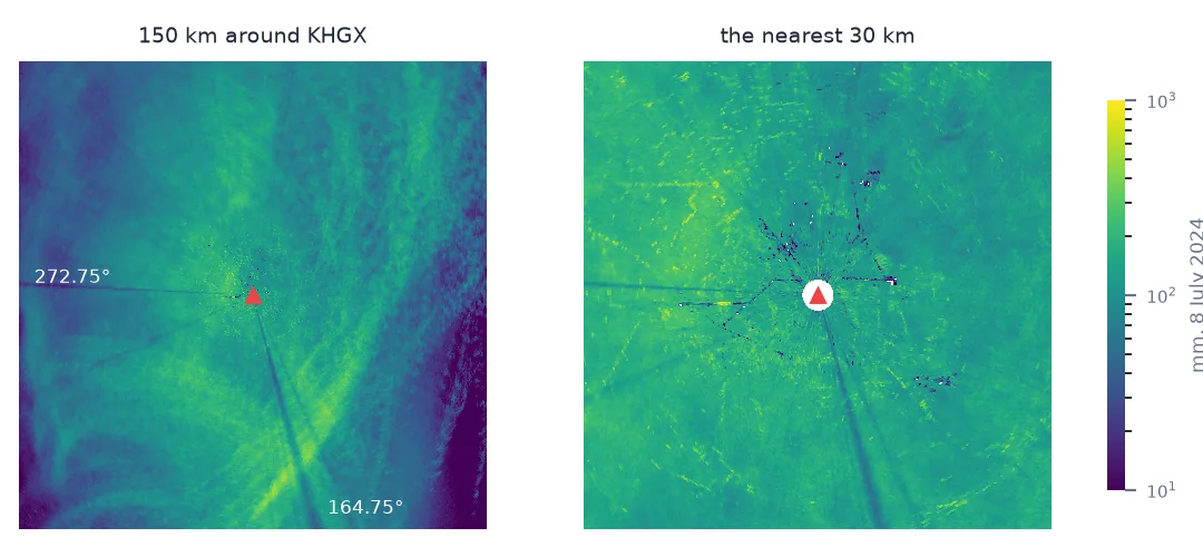
You accumulate a day of radar reflectivity into a rainfall map and two kinds of artefact appear. Thin wedges run outward from the radar with half the rain of the ground on either side — spokes. And close to the radar, isolated pixels hold several times the rain of their neighbours, some over a metre in a day — hot spots. Neither is weather. Spokes come from something blocking part of the beam; hot spots come from the beam hitting fixed targets on the ground. Both are permanent features of a given radar site, so they repeat in every accumulation you make.

This page finds both in a day of KHGX Level III reflectivity from 8 July 2024, when Hurricane Beryl crossed Houston, confirms what they are, and repairs them.

Quick answer

Average the day total over a ring of ranges for each azimuth and compare each ray with its neighbours. A blocked ray is a narrow dip:

ring = (RANGE > 30e3) & (RANGE < 120e3)
by_az = TOTAL[:, ring].mean(axis=1)
expected = median_filter(by_az, size=21, mode="wrap")              # 10° running median
deficit = by_az / expected
for i in np.argsort(deficit)[:6]:
    print(f"azimuth {AZ[i]:6.2f}: {by_az[i]:5.0f} mm against {expected[i]:4.0f} mm nearby ({deficit[i]:.0%})")

azimuth 164.75:    82 mm against  172 mm nearby (47%)
azimuth 165.25:    88 mm against  172 mm nearby (51%)
azimuth 164.25:    89 mm against  172 mm nearby (52%)
azimuth 272.75:    50 mm against   97 mm nearby (52%)
azimuth 165.75:   105 mm against  172 mm nearby (61%)
azimuth 163.75:   110 mm against  172 mm nearby (64%)

Find spokes, confirm blockage, find clutter

1. Find the spokes

The quick answer ranks every half-degree ray by how much rain it carries compared with the rays around it. Two groups stand out: around 164–166°, where rays receive half of what their neighbours do, and a single ray at 272.75°. A real rain band is never half a degree wide and dead straight through 120 km of the storm — these are features of the radar's surroundings.

2. Confirm it is blockage: where does it start, and does it fade higher up?

Two checks separate blockage from weather. A blocked ray is short of rain from the obstacle outward at every range, and the deficit shrinks or vanishes at a higher tilt that clears the obstacle:

def ratio_by_range(total, az, step=25):
    i = int(np.argmin(np.abs(AZ - az)))
    nb = (total[i - 6] + total[i + 6]) / 2                             # 3° either side
    return [f"{lo}-{lo + step} km: {total[i, (RANGE >= lo * 1e3) & (RANGE < (lo + step) * 1e3)].mean() / nb[(RANGE >= lo * 1e3) & (RANGE < (lo + step) * 1e3)].mean():.2f}"
            for lo in range(0, 150, step)]

for az in (164.75, 272.75):
    print(az, "; ".join(ratio_by_range(TOTAL, az)))

164.75 0-25 km: 0.43; 25-50 km: 0.40; 50-75 km: 0.38; 75-100 km: 0.42; 100-125 km: 0.43; 125-150 km: 0.42
272.75 0-25 km: 0.49; 25-50 km: 0.51; 50-75 km: 0.52; 75-100 km: 0.49; 100-125 km: 0.50; 125-150 km: 0.48

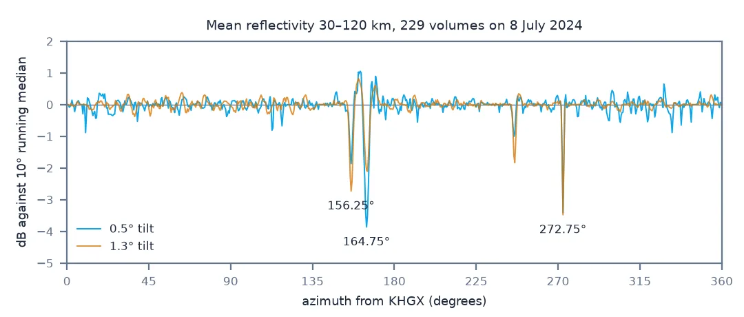
The deficit begins in the first range bin and stays roughly constant for 150 km: whatever cuts the beam is very close to the radar. Then compare the 0.5° tilt with the 1.3° tilt over the same scans, using mean reflectivity in decibels:

def az_deficit_db(mean_z):
    rng = (np.arange(mean_z.shape[1]) + 0.5) * 250.0
    db = 10 * np.log10(mean_z[:, (rng > 30e3) & (rng < 120e3)].mean(axis=1))
    return db - median_filter(db, size=21, mode="wrap")

d05, d13 = az_deficit_db(MEAN_Z[0.5]), az_deficit_db(MEAN_Z[1.3])
for az in (156.25, 164.75, 165.25, 272.75):
    i = int(np.argmin(np.abs(AZ - az)))
    print(f"{az:6.2f}: {d05[i]:+.1f} dB at 0.5 deg, {d13[i]:+.1f} dB at 1.3 deg")

156.25: -1.9 dB at 0.5 deg, -2.7 dB at 1.3 deg
164.75: -3.9 dB at 0.5 deg, -2.1 dB at 1.3 deg
165.25: -3.5 dB at 0.5 deg, -2.1 dB at 1.3 deg
272.75: -3.4 dB at 0.5 deg, -3.5 dB at 1.3 deg

At 164.75° the deficit almost halves at the higher tilt — partial blockage of the lowest beam. At 272.75° it does not change: the obstruction is tall enough to cut both tilts, and the ray needs a correction from its neighbours rather than from the next tilt up. And at 156.25° the deficit is larger at 1.3° than at 0.5° — something cuts the upper part of the beam there — which is a reminder that the next tilt up is not automatically clean.

3. Find the hot spots

Ground clutter is the opposite problem: a fixed target returns strong echo scan after scan, and the accumulation counts it as rain every time. Compare each gate with the median of its 5 × 9 neighbourhood:

local = median_filter(TOTAL, size=(5, 9), mode="wrap")
hot = (TOTAL > 3 * local) & (TOTAL > 200)
rows, cols = np.nonzero(hot)
print(f"{hot.sum()} hot gates, {(RANGE[cols] < 30e3).sum()} of them within 30 km; "
      f"worst {TOTAL.max():,.0f} mm at {AZ[np.unravel_index(TOTAL.argmax(), TOTAL.shape)[0]]:.2f} deg, "
      f"{RANGE[np.unravel_index(TOTAL.argmax(), TOTAL.shape)[1]] / 1000:.1f} km")
print(f"gates over 800 mm: {(TOTAL > 800).sum()}, all between {RANGE[np.nonzero(TOTAL > 800)[1]].min() / 1000:.1f} "
      f"and {RANGE[np.nonzero(TOTAL > 800)[1]].max() / 1000:.1f} km")
cold = (TOTAL < 0.3 * local) & (local > 50)
print(f"unusually dry gates: {cold.sum()}, {(RANGE[np.nonzero(cold)[1]] < 30e3).sum()} of them within 30 km")

42 hot gates, 39 of them within 30 km; worst 1,791 mm at 265.75 deg, 11.9 km
gates over 800 mm: 9, all between 9.4 and 18.4 km
unusually dry gates: 625, 616 of them within 30 km

Hot spots cluster close to the radar, where the lowest beam is only a few hundred metres up and meets towers, buildings and tree lines. The worst gate, 1,791 mm, is about five times the 369 mm that MRMS put in the wettest cell of the whole storm.

4. Repair the map

Interpolate blocked rays from their neighbours, and replace hot gates with the local median:

fixed = TOTAL.copy()
fixed[hot] = local[hot]
for az in (163.75, 164.25, 164.75, 165.25, 165.75, 272.75):
    i = int(np.argmin(np.abs(AZ - az)))
    fixed[i] = (fixed[i - 6] + fixed[i + 6]) / 2                      # 3° either side
by_az_fixed = fixed[:, ring].mean(axis=1)
for az in (164.75, 272.75):
    i = int(np.argmin(np.abs(AZ - az)))
    print(f"{az}: {by_az[i]:.0f} mm -> {by_az_fixed[i]:.0f} mm ({expected[i]:.0f} expected)")
print(f"maximum gate {TOTAL.max():,.0f} mm -> {fixed.max():,.0f} mm")

164.75: 82 mm -> 196 mm (172 expected)
272.75: 50 mm -> 99 mm (97 expected)
maximum gate 1,791 mm -> 778 mm

The 164.75° ray now carries a little more than the ±5° median, because its ±3° neighbours lie in a wetter band. The largest remaining gate, 778 mm at 317.75° and 19 km, sits in a cluster of strong gates, which lifts its local median until it is only 2.8 times that median — just under the threshold. A neighbourhood test misses clutter that covers several gates, and a lower multiplier starts to flag real convective cores. This is the simplest repair that works for a one-off map. Production systems do it better: MRMS uses a terrain-based blockage model to pick the lowest unblocked tilt for every gate, and clutter is removed in the radar's signal processor before reflectivity is recorded.

Checking a hot spot with dual-pol data

The data used on this page

NOAA NEXRAD Level III N0B and N1B (0.5° and 1.3° super-resolution base reflectivity) for KHGX, 8 July 2024, from the Unidata NEXRAD Level III archive on AWS, read with MetPy. The day total uses one 0.5° scan per volume (the one that starts the volume, matched to the 1.3° scan times) and a tropical Z = 250R¹·² relationship.

import datetime as dt
import re
import warnings
from pathlib import Path

import numpy as np
import requests
from metpy.io import Level3File
from scipy.ndimage import median_filter

warnings.filterwarnings("ignore")                   # MetPy warns about trailing bytes in some products
L3 = "https://unidata-nexrad-level3.s3.amazonaws.com/"


def keys(product):
    out, token = [], None
    while True:
        params = {"list-type": 2, "prefix": f"HGX_{product}_2024_07_08_"}
        if token:
            params["continuation-token"] = token
        text = requests.get(L3, params=params, timeout=60).text
        out += re.findall(r"<Key>([^<]+)</Key>", text)
        token = (re.findall(r"<NextContinuationToken>([^<]+)<", text) or [None])[0]
        if not token:
            return out


def read(key, folder):
    path = Path("data", folder, key)
    path.parent.mkdir(parents=True, exist_ok=True)
    if not path.exists():
        path.write_bytes(requests.get(L3 + key, timeout=60).content)
    try:
        f = Level3File(str(path))
        d = f.sym_block[0][0]
        return np.array(f.map_data(d["data"]), float)[np.argsort(d["start_az"])], f.metadata["vol_time"]
    except Exception:
        return None, None


n1b = keys("N1B")
volume_starts = {k[8:] for k in n1b}
MEAN_Z, TIMES, SCANS = {}, [], []
for tilt, product, folder in ((0.5, "N0B", "l3"), (1.3, "N1B", "l3n1")):
    acc, n = None, 0
    for key in (k for k in (n1b if product == "N1B" else keys("N0B")) if k[8:] in volume_starts):
        z, t = read(key, folder)
        if z is None or z.shape[0] != 720:
            continue
        lin = np.where(np.isfinite(z), 10 ** (z / 10), 0.0)
        acc = lin if acc is None else acc + lin
        n += 1
        if tilt == 0.5:
            SCANS.append(z); TIMES.append(t)
    MEAN_Z[tilt] = acc / n
AZ = np.arange(720) * 0.5 + 0.25
RANGE = (np.arange(1840) + 0.5) * 250.0
hours = np.diff([*TIMES, dt.datetime(2024, 7, 9)]) / dt.timedelta(hours=1)
TOTAL = np.zeros((720, 1840))
for z, h in zip(SCANS, hours):
    rate = (10 ** (np.nan_to_num(np.minimum(z, 53), nan=-30) / 10) / 250) ** (1 / 1.2)   # cap at 53 dBZ
    TOTAL += np.where(np.nan_to_num(z, nan=-30) > 5, rate, 0) * h
print(f"{len(SCANS)} volumes at 0.5 deg, {len(n1b)} at 1.3 deg; day total max {TOTAL.max():,.0f} mm")

229 volumes at 0.5 deg, 230 at 1.3 deg; day total max 1,791 mm

Example 1: check a hot spot against the dual-pol correlation coefficient

The worst hot gate should look like a ground target in a single Level II scan as well: ρhv well below rain's 0.97.

import xradar as xd
L2 = "2024/07/08/KHGX/KHGX20240708_090125_V06"
p2 = Path("data") / L2.split("/")[-1]
if not p2.exists():
    p2.write_bytes(requests.get("https://unidata-nexrad-level2.s3.amazonaws.com/" + L2, timeout=300).content)
sw = xd.io.open_nexradlevel2_datatree(str(p2))["sweep_0"].ds
i_hot, j_hot = np.unravel_index(TOTAL.argmax(), TOTAL.shape)
ii = int(np.argmin(np.abs(sw.azimuth.values - AZ[i_hot])))
jj = int(np.argmin(np.abs(sw.range.values - RANGE[j_hot])))
window = (slice(ii - 1, ii + 2), slice(jj - 2, jj + 3))
print(f"at {AZ[i_hot]:.2f} deg, {RANGE[j_hot] / 1000:.1f} km, 09:01 UTC: "
      f"Z {np.nanmax(sw.DBZH.values[window]):.0f} dBZ, rho_hv min {np.nanmin(sw.RHOHV.values[window]):.2f}")

at 265.75 deg, 11.9 km, 09:01 UTC: Z 47 dBZ, rho_hv min 0.56

A correlation coefficient of 0.56 under 47 dBZ is not rain: it is a ground target, and it was returning echo in the middle of a hurricane.

Example 2: how much of the day total do the artefacts change?

area = RANGE[None, :] * np.ones((720, 1))                           # gate area grows with range
inside = (RANGE[None, :] < 150e3) * np.ones((720, 1), bool)
mean_before = (TOTAL * area)[inside].sum() / area[inside].sum()
mean_after = (fixed * area)[inside].sum() / area[inside].sum()
print(f"area-mean within 150 km: {mean_before:.1f} mm before, {mean_after:.1f} mm after ({mean_after / mean_before - 1:+.1%})")

area-mean within 150 km: 103.6 mm before, 104.3 mm after (+0.6%)

The artefacts barely change an area average — they matter locally, to anyone who looks up the rain on their own street, a gauge site under a spoke, or a hydrologist modelling a small catchment that happens to lie under one.

A beam near the horizon

A radar beam near the horizon is a cone about a degree wide that starts at the antenna and passes only a few hundred metres above the ground for the first tens of kilometres. Anything that sticks into that cone — a tower, a building, a stand of trees — does two things. It reflects energy straight back, which appears as a strong, stationary echo at its range: clutter. And it takes energy out of the beam beyond it, so everything downrange in that direction looks weaker: blockage. One obstacle can do both, though on this map they do not line up: the strongest clutter gate, 1,791 mm at 11.9 km on 265.75°, is 7° away from the 272.75° spoke.

Signal processing removes most clutter before it is recorded, by filtering targets with zero Doppler velocity, but the filter also removes some rain and leaves the occasional speck — 616 of the 625 unusually dry gates on this map lie within 30 km, most likely gates where filtering took out rain along with the clutter. Blockage cannot be filtered: the energy never reached the rain. It can only be compensated, from a higher tilt, from neighbouring rays, or from a blockage model of the terrain and structures around the site.

Permanent blockage, propagation and wind farms

• Blockage is permanent per site: build a correction once from a long accumulation, then reuse it.
• A season-long total is a better detector than one storm: real rain bands average out.
• Anomalous propagation creates clutter that is not permanent, on stable nights and over the sea.
• Wind farms create clutter that moves, so Doppler filtering does not remove it.
• Partial blockage under about 50% is usually corrected by scaling; above that, use a higher tilt.
• Higher tilts trade blockage for height: at 100 km the 1.3° beam is already 2.9 km up.

Internal links

• How to estimate rainfall from radar — where this day total comes from
• Weather radar reflectivity explained — beam height and tilts
• Dual-polarisation radar explained — ρhv as a clutter test
• How to compare radar rainfall with gauges — when a gauge sits under a spoke
• How to read MRMS rainfall in Python — a product that corrects blockage

FAQ

Why does my radar rainfall map have lines radiating from the radar?

Those are blockage spokes: something near the radar — a tower, building or terrain — blocks part of the beam on those azimuths, so everything beyond looks drier.

What causes very high rainfall spots near a radar?

Ground clutter: fixed targets reflecting strongly in every scan, so the accumulation counts them as rain over and over.

How do I correct beam blockage?

Use a higher tilt where the obstacle is cleared, interpolate from neighbouring azimuths, or apply a blockage fraction from a terrain model, as MRMS does.

Can dual-pol data identify clutter?

Yes: ground targets have low correlation coefficient (ρhv), well below the 0.97 of rain.