
Radar Rainfall Too High: Hail and the Bright Band
On this page
Problem statement
Your radar rainfall estimate is far above what the gauges caught — not by a few percent but by a factor of two or ten, in a compact patch. Two physical causes produce this, and neither is a bug in your code. Hail is a strong reflector: a core of 65–75 dBZ turned into rain by a Z–R relationship becomes 200–1,000 mm/h, rain no storm produces. And the bright band — the layer where snow melts into rain — reflects more strongly than the snow above or the rain below, so wherever the beam passes through it, every gate looks wetter than the rain reaching the ground.
This page measures both in real radar data: the Denver hailstorm of 8 May 2017 from the KFTG radar, checked against 155 rain gauges, and the melting layer in Hurricane Beryl's rain from KHGX on 8 July 2024, checked against a radiosonde.
Quick answer
Cap reflectivity before converting it to rain, as NEXRAD's own precipitation processing does at 53 dBZ by default, and compare with gauges:
for name in ("nocap", "cap"):
    print(f"{name:5s}: radar/gauge {g[name].sum() / g.PRCP.sum():.2f}, mean bias {(g[name] - g.PRCP).mean():+.1f} mm, "
          f"r = {np.corrcoef(g[name], g.PRCP)[0, 1]:.2f}")
nocap: radar/gauge 1.75, mean bias +13.0 mm, r = 0.41
cap : radar/gauge 0.93, mean bias -1.2 mm, r = 0.49
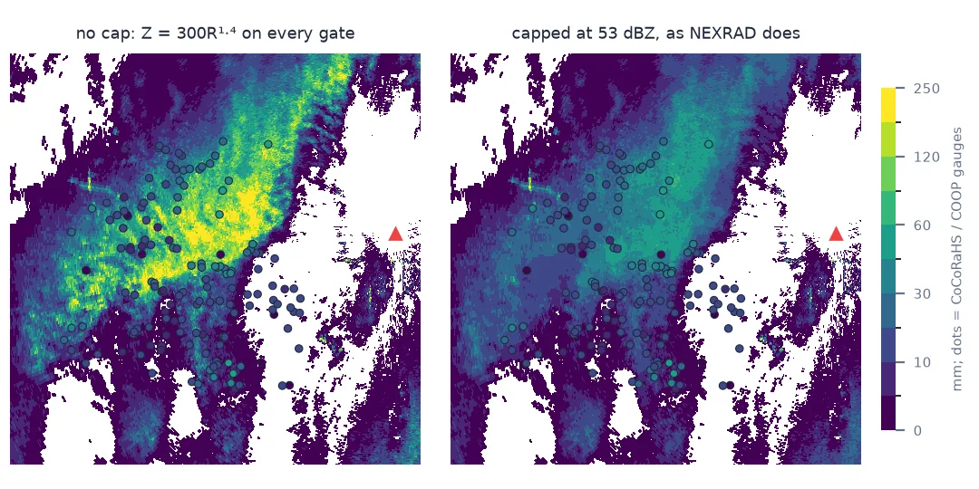
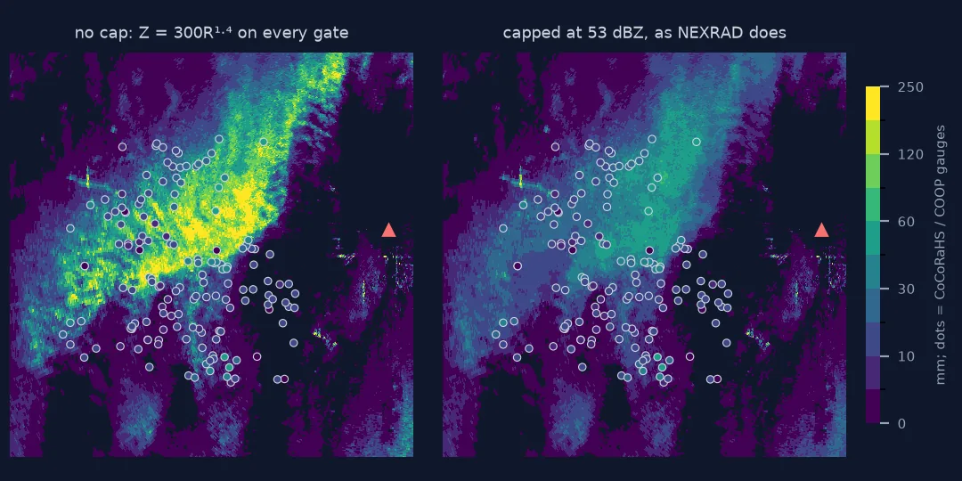
Recognise hail, see what Z-R does with it, cap and accumulate
1. Recognise hail in the radar data
Hail has a dual-polarisation fingerprint: very high reflectivity, differential reflectivity near zero because tumbling stones look round on average, and a correlation coefficient a little below that of pure rain. Compare the hail core with heavy rain in the same scan:
sw = xd.io.open_nexradlevel2_datatree(str(FILES[HAIL_SCAN]), sweep=[0])["sweep_0"].ds
z, zdr, rho = sw.DBZH.values, sw.ZDR.values, sw.RHOHV.values
for label, m in (("40-50 dBZ (rain)", (z >= 40) & (z < 50)), (">= 55 dBZ (hail core)", z >= 55)):
    print(f"{label:22s}: {m.sum():5d} gates, median ZDR {np.nanmedian(zdr[m]):5.2f} dB, "
          f"median rho_hv {np.nanmedian(rho[m]):.3f}, max Z {np.nanmax(z[m]):.0f}")
40-50 dBZ (rain) : 8340 gates, median ZDR 0.88 dB, median rho_hv 0.988, max Z 50
>= 55 dBZ (hail core) : 2457 gates, median ZDR 0.00 dB, median rho_hv 0.982, max Z 76
Rain at 40–50 dBZ has large, flattened drops and a ZDR well above zero. The hail core is far more reflective, yet its ZDR is lower: the extra reflectivity is not coming from more rain.
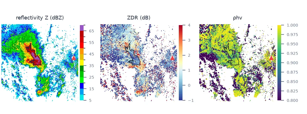
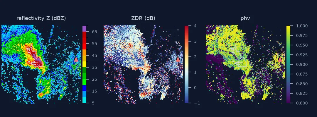
2. See what a Z–R relationship does with a hail core
for dbz in (45, 53, 60, 65, 72.5):
    print(f"{dbz:5.1f} dBZ -> {(10 ** (dbz / 10) / 300) ** (1 / 1.4):6.0f} mm/h")
45.0 dBZ -> 28 mm/h
53.0 dBZ -> 104 mm/h
60.0 dBZ -> 328 mm/h
65.0 dBZ -> 747 mm/h
72.5 dBZ -> 2566 mm/h
Every 5 dBZ above 53 more than doubles the rain rate. A single five-minute scan at 72.5 dBZ adds about 210 mm — more than four times what the wettest gauge in the metro, 48 mm, caught all day.
3. Accumulate with and without the cap and check against gauges
The quick answer compares the two storm totals at every gauge. The gauges under the hail core show where the difference comes from:
core = g[g.zmax >= 60].sort_values("nocap", ascending=False)
print(f"{len(core)} gauges under at least 60 dBZ: gauge {core.PRCP.mean():.1f} mm, "
      f"radar {core.nocap.mean():.1f} mm uncapped, {core.cap.mean():.1f} mm capped")
print(core.head(5)[["NAME", "PRCP", "nocap", "cap", "zmax"]].round(1).to_string(index=False))
31 gauges under at least 60 dBZ: gauge 23.2 mm, radar 93.3 mm uncapped, 32.4 mm capped
NAME PRCP nocap cap zmax
ARVADA 2.1 SSE, CO US 9.1 218.0 23.5 72.5
DENVER 6.1 WSW, CO US 33.0 191.9 36.0 67.0
LAKEWOOD 1.2 E, CO US 27.2 145.8 26.6 66.5
COMMERCE CITY 1.2 WNW, CO US 48.3 134.4 46.5 64.5
DENVER WATER DEPARTMENT, CO US 31.2 128.8 29.0 65.5
Without the cap the radar is four times the gauges under the core, and 24 times at the worst gauge. The cap removes most of that, but not all: even capped, these gauges get 40% more from the radar than they caught. The cap is a blunt instrument — it also clips genuinely heavy rain, which is why dual-pol rainfall algorithms switch to a KDP-based relationship in hail instead.
4. Find the bright band in a vertical profile
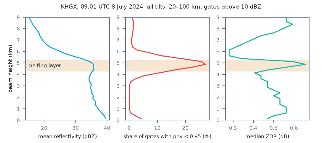
Melting snowflakes are large, wet and irregular: they reflect like big raindrops, they flatten into higher ZDR, and their mix of shapes lowers ρhv. Build a vertical profile from every tilt of one volume:
H, Z, RH, ZD = [], [], [], []
for angle, name in tilts.items():
    ds = vol[name].ds
    if "RHOHV" not in ds:
        continue
    r = ds.range.values / 1000
    near = (r > 20) & (r < 100)
    h = np.broadcast_to(beam_height(r, angle)[None, :], ds.DBZH.shape)[:, near]
    zz = ds.DBZH.values[:, near]
    ok = zz > 10
    H.append(h[ok]); Z.append(zz[ok]); RH.append(ds.RHOHV.values[:, near][ok]); ZD.append(ds.ZDR.values[:, near][ok])
H, Z, RH, ZD = map(np.concatenate, (H, Z, RH, ZD))
for lo in np.arange(2.5, 7.0, 0.5):
    m = (H >= lo) & (H < lo + 0.5)
    print(f"{lo:.1f}-{lo + 0.5:.1f} km: mean {10 * np.log10(np.mean(10 ** (Z[m] / 10))):4.1f} dBZ, "
          f"rho_hv < 0.95 in {np.mean(RH[m] < 0.95):4.0%}, median ZDR {np.nanmedian(ZD[m]):.2f}")
print(f"0 C at Lake Charles, 12 UTC: {zero_c:,.0f} m")
2.5-3.0 km: mean 34.8 dBZ, rho_hv < 0.95 in 0%, median ZDR 0.50
3.0-3.5 km: mean 34.7 dBZ, rho_hv < 0.95 in 0%, median ZDR 0.47
3.5-4.0 km: mean 34.4 dBZ, rho_hv < 0.95 in 4%, median ZDR 0.44
4.0-4.5 km: mean 35.3 dBZ, rho_hv < 0.95 in 13%, median ZDR 0.44
4.5-5.0 km: mean 35.7 dBZ, rho_hv < 0.95 in 25%, median ZDR 0.59
5.0-5.5 km: mean 33.4 dBZ, rho_hv < 0.95 in 22%, median ZDR 0.47
5.5-6.0 km: mean 27.7 dBZ, rho_hv < 0.95 in 10%, median ZDR 0.28
6.0-6.5 km: mean 23.2 dBZ, rho_hv < 0.95 in 2%, median ZDR 0.28
6.5-7.0 km: mean 20.3 dBZ, rho_hv < 0.95 in 1%, median ZDR 0.34
0 C at Lake Charles, 12 UTC: 4,653 m
All three fields agree on a layer at about 4.5–5 km, and the nearest radiosonde, 190 km to the east, puts the freezing level at 4,653 m — inside it. In Beryl's tropical rain the bright band is weak — a dBZ or so above the rain below it — because the rain is dominated by warm-cloud processes, but the ρhv signature is unmistakable.
5. Find where the lowest beam crosses it
for edge in (4.25, 5.25):
    r = brentq(lambda rr: beam_height(rr, 0.48) - edge, 1, 400)
    print(f"0.48 deg beam centre reaches {edge} km at {r:.0f} km range")
0.48 deg beam centre reaches 4.25 km at 207 km range
0.48 deg beam centre reaches 5.25 km at 236 km range
Beyond that range, the lowest tilt samples melting snow and then snow, not rain. Rainfall estimates there need a vertical-profile correction, or should come from a closer radar.
How much of the overestimate is the hail core
The data used on this page
NOAA NEXRAD Level II from the Unidata archive on AWS: KFTG (Denver), every volume from 19:00 to 23:00 UTC on 8 May 2017, and KHGX, 09:01 UTC on 8 July 2024. Daily precipitation for 9 May 2017 (the 24 hours ending that morning) from the NCEI daily-summaries service — mostly CoCoRaHS volunteer gauges. The Lake Charles (72240) radiosonde from the University of Wyoming sounding archive.
import datetime as dt
import io
import re
from pathlib import Path

import numpy as np
import pandas as pd
import requests
import xradar as xd
from pyproj import Geod
from scipy.optimize import brentq

Path("data/kftg").mkdir(parents=True, exist_ok=True)
L2 = "https://unidata-nexrad-level2.s3.amazonaws.com/"
FILES = []
for hour in ("19", "20", "21", "22"):
    listing = requests.get(L2, params={"list-type": 2, "prefix": f"2017/05/08/KFTG/KFTG20170508_{hour}"}, timeout=60).text
    for key in (k for k in re.findall(r"<Key>([^<]+)</Key>", listing) if k.endswith("_V06")):
        path = Path("data/kftg") / key.split("/")[-1]
        if not path.exists():
            path.write_bytes(requests.get(L2 + key, timeout=300).content)
        FILES.append(path)
HAIL_SCAN = [p.name for p in FILES].index("KFTG20170508_211531_V06")

API = "https://www.ncei.noaa.gov/access/services"
found = requests.get(f"{API}/search/v1/data", params={"dataset": "daily-summaries", "bbox": "39.95,-105.3,39.5,-104.75",
                     "startDate": "2017-05-09T00:00:00", "endDate": "2017-05-09T23:59:59", "dataTypes": "PRCP", "limit": 1000}, timeout=120).json()
ids = sorted({s["id"] for res in found["results"] for s in res["stations"]})
g = pd.concat(pd.read_csv(io.StringIO(requests.get(f"{API}/data/v1", params={
    "dataset": "daily-summaries", "stations": ",".join(ids[i:i + 100]), "startDate": "2017-05-09", "endDate": "2017-05-09",
    "dataTypes": "PRCP", "format": "csv", "includeStationLocation": "1", "includeStationName": "true", "units": "metric"},
    timeout=120).text)) for i in range(0, len(ids), 100)).dropna(subset=["PRCP"]).reset_index(drop=True)

# storm total at each gauge from the 0.5 deg tilt, Z = 300 R^1.4, with and without the 53 dBZ cap
az, _, dist = Geod(ellps="WGS84").inv(np.full(len(g), -104.5458), np.full(len(g), 39.7866), g.LONGITUDE.values, g.LATITUDE.values)
times = [dt.datetime.strptime(p.name[4:19], "%Y%m%d_%H%M%S") for p in FILES]
hours = np.diff([*times, times[-1] + dt.timedelta(minutes=5)]) / dt.timedelta(hours=1)
rate = lambda dbz: np.where(dbz > 5, (10 ** (dbz / 10) / 300) ** (1 / 1.4), 0.0)
g["cap"] = g["nocap"] = 0.0
g["zmax"] = -30.0
for path, h in zip(FILES, hours):
    s0 = xd.io.open_nexradlevel2_datatree(str(path), sweep=[0])["sweep_0"].ds
    i = np.array([np.argmin(np.abs((s0.azimuth.values - a + 180) % 360 - 180)) for a in az % 360])
    j = np.searchsorted(s0.range.values, dist).clip(0, s0.sizes["range"] - 1)
    zg = np.nan_to_num(s0.DBZH.values[i, j], nan=-30)
    g["zmax"] = np.maximum(g.zmax, zg)
    g["cap"] += rate(np.minimum(zg, 53)) * h
    g["nocap"] += rate(zg) * h

KEY = "2024/07/08/KHGX/KHGX20240708_090125_V06"
khgx = Path("data") / KEY.split("/")[-1]
if not khgx.exists():
    khgx.write_bytes(requests.get(L2 + KEY, timeout=300).content)
vol = xd.io.open_nexradlevel2_datatree(str(khgx))
tilts = {}
for name in sorted((c for c in vol.children if c.startswith("sweep")), key=lambda c: int(c.split("_")[1])):
    tilts.setdefault(round(float(vol[name].ds.sweep_fixed_angle), 2), name)


def beam_height(r_km, elev_deg, ke=4 / 3, a=6371.0):
    return np.sqrt(r_km**2 + (ke * a) ** 2 + 2 * r_km * ke * a * np.sin(np.radians(elev_deg))) - ke * a


snd = pd.read_csv(io.StringIO(requests.get("https://weather.uwyo.edu/wsgi/sounding",
                  params={"datetime": "2024-07-08 12:00:00", "id": "72240", "type": "TEXT:CSV"}, timeout=120).text))
snd.columns = [c.strip() for c in snd.columns]
t, hgt = snd["temperature_C"].values, snd["geopotential height_m"].values
k = np.nonzero((t[:-1] > 0) & (t[1:] <= 0))[0][0]
zero_c = hgt[k] + (hgt[k + 1] - hgt[k]) * t[k] / (t[k] - t[k + 1])
print(f"{len(FILES)} KFTG volumes {times[0]:%H:%M}-{times[-1]:%H:%M} UTC; {len(g)} gauges, "
      f"{g.PRCP.min():.0f}-{g.PRCP.max():.0f} mm; {len(tilts)} KHGX tilts")
52 KFTG volumes 19:01-22:59 UTC; 155 gauges, 0-48 mm; 14 KHGX tilts
Example 1: how much of the overestimate is the hail core?
for lo, hi in ((-30, 55), (55, 60), (60, 80)):
    m = (g.zmax >= lo) & (g.zmax < hi)
    print(f"max Z {lo:>3}-{hi} dBZ: {m.sum():3d} gauges, radar/gauge {g.nocap[m].sum() / g.PRCP[m].sum():.2f} uncapped, "
          f"{g.cap[m].sum() / g.PRCP[m].sum():.2f} capped")
print("gauges reporting 0 mm under 55 dBZ or more:", g[(g.PRCP == 0) & (g.zmax >= 55)][["NAME", "zmax"]].values.tolist())
max Z -30-55 dBZ: 94 gauges, radar/gauge 0.52 uncapped, 0.51 capped
max Z 55-60 dBZ: 30 gauges, radar/gauge 1.96 uncapped, 1.41 capped
max Z 60-80 dBZ: 31 gauges, radar/gauge 4.02 uncapped, 1.40 capped
gauges reporting 0 mm under 55 dBZ or more: [['DENVER MUSEUM, CO US', 61.5]]
The overall ratio of 0.93 in the quick answer is two errors cancelling. Under the hail the capped radar is still 40% high; away from it, at the 94 gauges that never saw 55 dBZ, the radar has only half the gauge total. Part of that is the window: a CoCoRaHS day runs from 7 am to 7 am, and this page accumulates only the four hours of the storm. Part may be the Z–R relationship. The page does not separate the two, which is a reminder to compare over matched windows before tuning anything.
Example 2: a dual-pol hail flag instead of a blanket cap
hail = (z >= 50) & (zdr < 1.0)
print(f"{hail.sum()} gates flagged at 21:15 UTC; of the {(z >= 55).sum()} gates at 55 dBZ or more, "
      f"{(hail & (z >= 55)).sum() / (z >= 55).sum():.0%} are flagged, and {(hail & (z < 53)).sum()} flagged gates are below the cap")
3290 gates flagged at 21:15 UTC; of the 2457 gates at 55 dBZ or more, 81% are flagged, and 818 flagged gates are below the cap
The flag and the cap disagree on a lot of gates. A fifth of the gates at 55 dBZ or more escape the flag because their ZDR is above 1 dB, which is large drops or melting hail coated in water. And 818 flagged gates sit below the cap, where hail mixed with rain is already being counted as rain. At the margins, where hail and very large drops mix, no single rule is clean, which is why operational classifiers weigh several fields.
Why a few hailstones dominate reflectivity
A Z–R relationship assumes the targets are raindrops with a typical size distribution. Reflectivity grows with the sixth power of diameter, so a few large targets dominate it. A hailstone of 2–5 cm is a very large target. Its reflectivity is no guide to how much water reaches the ground, and that water arrives as ice that bounces out of gauges or melts slowly. The Denver storm was the costliest hailstorm in Colorado's history. On the radar it was a 70+ dBZ core over Lakewood, Wheat Ridge and Arvada. In the gauges it was an ordinary 10–30 mm.
The bright band is subtler. Above the 0 °C level, snow is a weak reflector because ice scatters about a fifth as strongly as water. As it falls through the melting layer, each flake gains a water coating while it is still large, and reflects like a giant raindrop. Then it collapses into a smaller drop and speeds up, and reflectivity drops again. A radar beam crossing that layer sees the peak. Close to the radar the lowest tilt is below the band; far away the beam rises through it, and a fixed Z–R relationship turns the bright band into a ring of exaggerated rain.
Gauge undercatch, gauge days and winter bright bands
- Gauges undercatch hail: stones bounce out, and some observers do not melt and measure them. One gauge under 61.5 dBZ reported 0.0 mm.
- The gauge day is longer than the radar window: CoCoRaHS totals run 7 am to 7 am local time; this page's radar covers 19–23 UTC, the storm itself.
- Winter bright bands are lower and stronger, often at 1–2 km, and dominate cool-season radar errors.
- KDP is immune to hail to first order, which is why dual-pol algorithms use R(KDP) in hail cores.
- The 53 dBZ cap is a site parameter; some radars use a different value.
- A sounding 190 km away gives the freezing level only approximately; the radar's own ρhv dip is local.
Internal links
- How to estimate rainfall from radar — Z–R relationships and the cap
- Dual-polarisation radar explained — ZDR and ρhv
- Weather radar reflectivity explained — beam height and tilts
- How to compare radar rainfall with gauges — matching windows
- Radar beam blockage and clutter — the other artefacts
FAQ
Why is radar rainfall too high in hailstorms?
Hail reflects far more strongly than the rain it contains. A Z–R relationship turns 70 dBZ into hundreds of millimetres per hour. In the Denver 2017 storm the uncapped radar total was 218 mm at a gauge that caught 9 mm.
What is the 53 dBZ hail cap?
NEXRAD rainfall processing limits reflectivity to 53 dBZ before converting it to rain, so hail cores cannot produce absurd rates.
What is the radar bright band?
The layer where snow melts into rain. Wet, large melting flakes reflect strongly, raising reflectivity and ZDR and lowering ρhv. In Beryl it was at 4.5–5 km.
How do I correct for the bright band?
Use the lowest tilt that is below it, apply a vertical-profile-of-reflectivity correction, or take rainfall from a closer radar.