How to Estimate Rainfall from Radar Reflectivity in Python

Problem statement

A weather radar measures reflectivity, not rain. Turning one into the other uses a Z–R relationship, Z = aR^b, whose two constants depend on the size of the raindrops — and drop sizes in a tropical cyclone are nothing like those in a Midwest thunderstorm. Choose the wrong pair and a day's rainfall comes out at half its true value. Then the rates have to be summed through time, from scans that are not evenly spaced, and a few gates that echo off buildings every scan can pile up implausible totals.

This page accumulates 24 hours of lowest-tilt reflectivity from the KHGX (Houston) radar on 8 July 2024, the day Hurricane Beryl came ashore, with three standard Z–R relationships, and compares each with the gauge-corrected MRMS total for the same day.

Quick answer

Convert each scan's dBZ to linear Z, cap it to keep hail out, invert Z = aR^b for rain rate, and multiply by the time until the next scan:

def rain_rate(dbz, a, b, cap=53.0):
    """mm/h from dBZ via Z = a R^b; echoes below 5 dBZ are no rain, above `cap` are capped (hail)."""
    d = np.nan_to_num(dbz, nan=-99.0)
    r = (10 ** (np.minimum(d, cap) / 10) / a) ** (1 / b)
    return np.where(d >= 5, r, 0.0)

ZR = {"Marshall-Palmer": (200, 1.6), "WSR-88D convective": (300, 1.4), "tropical": (250, 1.2)}
totals = {}
for name, (a, b) in ZR.items():
    totals[name] = sum(rain_rate(dbz, a, b) * hours for dbz, hours in zip(SCANS, HOURS))
for name, tot in totals.items():
    s = tot[RING]
    print(f"{name:20} 24 h total vs MRMS: ratio {s[OK].sum() / MRMS_AT[OK].sum():.2f}, r {np.corrcoef(s[OK], MRMS_AT[OK])[0, 1]:.2f}")

Marshall-Palmer      24 h total vs MRMS: ratio 0.54, r 0.88
WSR-88D convective   24 h total vs MRMS: ratio 0.56, r 0.87
tropical             24 h total vs MRMS: ratio 1.01, r 0.84

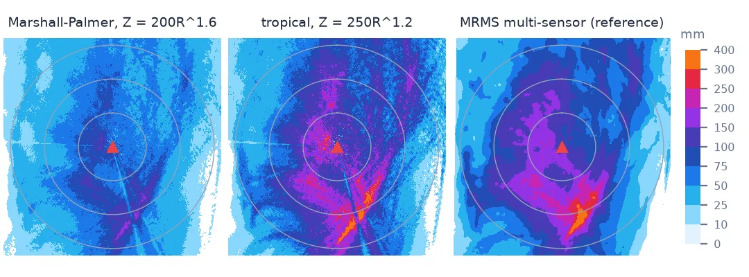
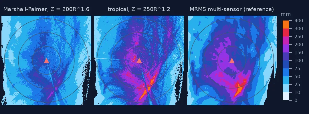
A day of low-tilt reflectivity, a Z-R relationship, real time steps

1. Get a day of lowest-tilt reflectivity

The Level III product N0B is the 0.5° super-resolution reflectivity, about 0.3 MB per scan against 19 MB for a Level II volume. The radar also writes N0B for every supplemental low-level scan; selecting the scans that start a volume — the same times as the Level II files — gives one per volume:

print(len(SCANS), "volume scans;", TIMES[0], "to", TIMES[-1], f"; {UNREADABLE} files could not be parsed")
gaps = np.diff([t.timestamp() for t in TIMES]) / 60
print(f"spacing between scans: median {np.median(gaps):.1f} min, longest {gaps.max():.1f} min")

230 volume scans; 2024-07-08 00:01:25 to 2024-07-08 23:55:16 ; 1 files could not be parsed
spacing between scans: median 6.6 min, longest 13.8 min

2. Choose a Z–R relationship

Each relationship encodes a typical drop-size distribution. Marshall–Palmer (Z = 200R^1.6) was fitted to stratiform rain; the WSR-88D default (Z = 300R^1.4) to Plains convection; the tropical relationship (Z = 250R^1.2) to the many small drops of warm, maritime rain. At the same reflectivity they give very different rates:

for dbz in (30, 40, 50):
    print(f"{dbz} dBZ: " + ", ".join(f"{n} {rain_rate(np.array([dbz]), a, b)[0]:5.1f} mm/h" for n, (a, b) in ZR.items()))

30 dBZ: Marshall-Palmer   2.7 mm/h, WSR-88D convective   2.4 mm/h, tropical   3.2 mm/h
40 dBZ: Marshall-Palmer  11.5 mm/h, WSR-88D convective  12.2 mm/h, tropical  21.6 mm/h
50 dBZ: Marshall-Palmer  48.6 mm/h, WSR-88D convective  63.4 mm/h, tropical 147.4 mm/h

3. Accumulate with the real time steps

Each scan's rate applies until the next scan. Volumes are five to seven minutes apart in storm mode, but not exactly; using the actual intervals rather than an assumed one keeps the total honest. The quick answer's HOURS are those intervals, clipped to the day.

4. Compare with a reference

MRMS MultiSensor Pass2 for the 24 hours ending 00 UTC on 9 July — the same UTC day — is gauge-corrected and a reasonable reference. Comparing at each gate between 20 and 150 km from the radar, where MRMS has at least 5 mm:

The quick answer's ratios say it plainly: the two mid-latitude relationships produce barely more than half the gauge-corrected rain; the tropical relationship matches it in total. All three correlate well in pattern — reflectivity knows where the rain was — but only the tropical one knows how much.

5. Check for clutter

A total map should be looked at before it is used:

trop = totals["tropical"]
i = np.unravel_index(np.argmax(np.where(RANGE[None, :] < 150_000, trop, 0)), trop.shape)
print(f"largest tropical total: {trop[i]:,.0f} mm at azimuth {AZ[i[0]]:.2f}, range {RANGE[i[1]] / 1000:.1f} km")
print(f"99.9th percentile 20-150 km: {np.percentile(trop[:, (RANGE > 20e3) & (RANGE < 150e3)], 99.9):.0f} mm; "
      f"gates above 800 mm: {(trop > 800).sum()}")

largest tropical total: 1,792 mm at azimuth 265.75, range 11.9 km
99.9th percentile 20-150 km: 401 mm; gates above 800 mm: 9

Nine gates, all within 20 km of the radar on two bearings, carry totals several times the 99.9th percentile. They echo off fixed targets in every scan and accumulate them into "rain". Masking them — by range, by a clutter map, or by the dual-polarisation correlation coefficient — belongs before any total is reported (see beam blockage and clutter).

What the hail cap does

The data used on this page

NOAA NEXRAD Level III N0B (0.5° super-resolution base reflectivity) for KHGX, 8 July 2024, from the Unidata NEXRAD Level III archive on AWS, with volume times from the Level II listing; MRMS MultiSensor QPE Pass2, 24 hours ending 00 UTC 9 July 2024, from the NOAA MRMS archive on AWS. Read with MetPy and cfgrib.

import datetime as dt
import gzip
import re
import shutil
import warnings
from pathlib import Path

import numpy as np
import requests
import xarray as xr
from metpy.io import Level3File
from pyproj import Geod

warnings.filterwarnings("ignore")                   # MetPy warns about trailing bytes in some products
Path("data/l3").mkdir(parents=True, exist_ok=True)
L2 = "https://unidata-nexrad-level2.s3.amazonaws.com/"
L3 = "https://unidata-nexrad-level3.s3.amazonaws.com/"
listing = requests.get(L2, params={"list-type": 2, "prefix": "2024/07/08/KHGX/"}, timeout=60).text
vol_times = sorted({re.search(r"KHGX(\d{8})_(\d{6})_V06$", k).group(2) for k in re.findall(r"<Key>([^<]+)</Key>", listing)
                    if k.endswith("_V06")})
SCANS, TIMES, UNREADABLE = [], [], 0
for hms in vol_times:
    key = f"HGX_N0B_2024_07_08_{hms[:2]}_{hms[2:4]}_{hms[4:]}"
    path = Path("data/l3") / key
    if not path.exists():
        r = requests.get(L3 + key, timeout=60)
        if r.status_code != 200:
            continue
        path.write_bytes(r.content)
    try:
        f = Level3File(str(path))
        d = f.sym_block[0][0]
        order = np.argsort(d["start_az"])
        SCANS.append(np.array(f.map_data(d["data"]), float)[order])
        TIMES.append(f.metadata["vol_time"])
    except Exception:
        UNREADABLE += 1
day_end = dt.datetime(2024, 7, 9)
HOURS = [((TIMES[i + 1] if i + 1 < len(TIMES) else day_end) - t).total_seconds() / 3600 for i, t in enumerate(TIMES)]
AZ = np.arange(720) * 0.5 + 0.25
RANGE = (np.arange(1840) + 0.5) * 250.0                        # N0B gates start at the radar, every 250 m

name = "MRMS_MultiSensor_QPE_24H_Pass2_00.00_20240709-000000.grib2"
if not Path("data", name).exists():
    url = f"https://noaa-mrms-pds.s3.amazonaws.com/CONUS/MultiSensor_QPE_24H_Pass2_00.00/20240709/{name}.gz"
    Path("data", name + ".gz").write_bytes(requests.get(url, timeout=300).content)
    with gzip.open(Path("data", name + ".gz")) as fz, open(Path("data", name), "wb") as o:
        shutil.copyfileobj(fz, o)
mrms = xr.open_dataset(Path("data", name), engine="cfgrib", decode_timedelta=True, backend_kwargs={"indexpath": ""})["unknown"]
A2, R2 = np.meshgrid(AZ, RANGE, indexing="ij")
RING = (R2 > 20e3) & (R2 < 150e3)
lon, lat, _ = Geod(ellps="WGS84").fwd(np.full(RING.sum(), -95.0787), np.full(RING.sum(), 29.4719), A2[RING], R2[RING])
MRMS_AT = mrms.sel(latitude=xr.DataArray(lat, dims="p"), longitude=xr.DataArray(lon % 360, dims="p"), method="nearest").values
OK = np.isfinite(MRMS_AT) & (MRMS_AT >= 5)
print(len(SCANS), "scans")

230 scans

Example 1: what the hail cap does

Capping reflectivity at 53 dBZ limits the rate any one scan can contribute. Without it:

a, b = ZR["tropical"]
nocap = sum(rain_rate(d, a, b, cap=99) * h for d, h in zip(SCANS, HOURS))
print(f"tropical, no cap: ratio to MRMS {nocap[RING][OK].sum() / MRMS_AT[OK].sum():.2f}; "
      f"gates above 800 mm {(nocap > 800).sum()} (capped: {(totals['tropical'] > 800).sum()})")

tropical, no cap: ratio to MRMS 1.01; gates above 800 mm 54 (capped: 9)

Example 2: the totals by distance from the radar

The beam rises with range, so the radar sees rain higher up farther out:

for lo, hi in ((20, 60), (60, 100), (100, 150)):
    m = (R2[RING] > lo * 1e3) & (R2[RING] < hi * 1e3) & OK
    s = totals["tropical"][RING]
    print(f"{lo:3d}-{hi:3d} km: tropical / MRMS = {s[m].sum() / MRMS_AT[m].sum():.2f}")

 20- 60 km: tropical / MRMS = 1.04
 60-100 km: tropical / MRMS = 0.96
100-150 km: tropical / MRMS = 1.03

The ratio holds within 4% from 20 to 150 km. Beryl's rain was deep enough that even the rising beam stayed inside it; in shallow winter rain the far range would read low.

Reflectivity and rain rate scale differently with drop size

Reflectivity is proportional to the sum of the sixth powers of drop diameters in the sampled volume; rain rate depends roughly on the 3.7th power. The two are linked only through the drop-size distribution, so any Z–R relationship is a statement about what kind of rain is falling. Tropical cyclones produce large numbers of small drops: modest reflectivity, heavy rain. A relationship tuned for continental thunderstorms, with fewer, larger drops, reads the same reflectivity as much lighter rain.

That is why operational systems switch relationships by rain type — MRMS applies a tropical relationship where its classification finds tropical rain — and why a single default can be off by a factor of two in exactly the storms that matter most. The remaining steps are bookkeeping that is easy to get wrong: integrate with real scan intervals, cap the reflectivity so hail does not count as torrential rain, and inspect the result for gates that accumulate clutter.

Rain types, the hail cap and supplemental scans

• Pick Z–R by rain type: tropical for hurricanes and warm maritime rain.
• Cap at about 53 dBZ so hail does not become extreme rain.
• Use actual scan intervals, clipped to the accumulation window.
• Skip supplemental scans or weight them correctly; they are extra low-level looks.
• Inspect for clutter; persistent near-range echoes accumulate.
• Beam height grows with range; far-range totals sample rain aloft.

Internal links

• Weather radar reflectivity explained — what Z is
• How to read MRMS rainfall from GRIB2 — the reference used here
• Radar rainfall too high: hail and bright band — the opposite error
• Radar beam blockage and clutter — the gates to mask
• How to map storm-total rainfall — from totals to maps

FAQ

What Z-R relationship should I use?

It depends on the rain: Z = 200R^1.6 for stratiform rain, Z = 300R^1.4 for continental convection, Z = 250R^1.2 for tropical rain. For Hurricane Beryl the tropical relationship matched the gauge-corrected total; the others gave about half.

How do I convert dBZ to rain rate in Python?

Z = 10^(dBZ/10), then R = (Z/a)^(1/b) in mm/h; cap dBZ at about 53 first.

How do I accumulate radar rainfall over time?

Multiply each scan's rain rate by the time until the next scan (in hours) and sum, clipping the first and last intervals to the window.

Why is my radar rainfall total so high near the radar?

Ground clutter: fixed targets that echo in every scan accumulate into large totals. Mask them before summing.