How to Make a Weather Radar Loop Animation in Python

Problem statement

A radar loop, a sequence of reflectivity scans played as a short film, is the most direct way to show a storm moving. Building one from raw scans raises problems a single map never meets. Scans arrive at irregular intervals, so a fixed frame rate plays the storm at a changing speed. Drawing polar gates with pcolormesh for every frame is slow. The colour scale must stay fixed or the loop flickers. And the output format decides whether the result is 2 MB or 20.

This page builds a three-hour loop of Hurricane Beryl's landfall on 8 July 2024 from 95 NEXRAD Level III scans of the KHGX radar near Houston. It grids each scan once with a lookup table, paces the frames by real time, and compares GIF, MP4 and animated WebP.

Quick answer

Grid every scan through a precomputed polar-to-raster lookup, keep one colour scale for all frames, and give each frame a duration proportional to the time until the next scan:

frames = [np.where(VALID, z[AI, RI], np.nan) for _, z in SCANS]           # 1 km grid, 460 x 460 km
gap_min = pd.Series([t for t, _ in SCANS] + [SCANS[-1][0] + pd.Timedelta(minutes=2)]).diff().dropna().dt.total_seconds().to_numpy() / 60
images = [render(f, t) for f, (t, _) in zip(frames, SCANS)]               # same cmap and norm every time
durations = (gap_min * 60).round().astype(int).tolist()                   # ms per frame: 1 min of storm -> 60 ms
images[0].save("data/khgx_loop.gif", save_all=True, append_images=images[1:], duration=durations, loop=0)
print(f"{len(images)} frames, {sum(durations) / 1000:.1f} s of animation for {(SCANS[-1][0] - SCANS[0][0]).total_seconds() / 3600:.1f} h of storm; "
      f"{Path('data/khgx_loop.gif').stat().st_size / 1e6:.1f} MB")

95 frames, 10.8 s of animation for 3.0 h of storm; 3.1 MB

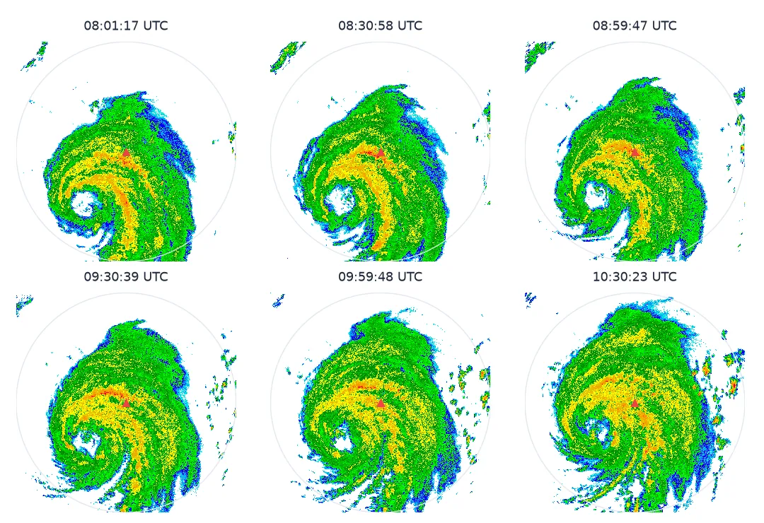
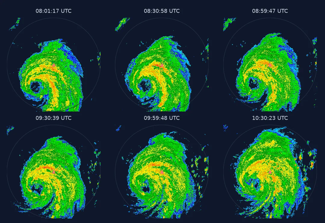
Read the timing, grid once, fix the colour scale, pace by real time

1. Look at the timing before animating

t = pd.Series([s[0] for s in SCANS])
gaps = t.diff().dt.total_seconds().dropna() / 60
print(f"{len(t)} scans from {t.iloc[0]:%H:%M} to {t.iloc[-1]:%H:%M} UTC; gaps min {gaps.min():.1f}, median {gaps.median():.1f}, max {gaps.max():.1f} min")
print("gap counts (min):", gaps.round().value_counts().sort_index().to_dict())

95 scans from 08:01 to 10:59 UTC; gaps min 1.2, median 1.8, max 3.4 min
gap counts (min): {1.0: 20, 2.0: 60, 3.0: 14}

The KHGX radar was scanning its lowest tilt several times per volume (SAILS), so 0.5° scans come one to three and a half minutes apart. Played at a fixed frame rate, the storm would appear to speed up and slow down for no meteorological reason.

2. Grid once, reuse for every frame

A Level III scan is 720 azimuths by 1,840 range gates. Drawing that as a polar mesh is accurate but slow. A lookup table from each output pixel to its azimuth and gate is computed once and applied to every scan as an index:

import os
import time
z = SCANS[0][1]
t0 = time.perf_counter(); g = np.where(VALID, z[AI, RI], np.nan); t_lookup = time.perf_counter() - t0
fig, ax = plt.subplots()
t0 = time.perf_counter(); ax.pcolormesh(PX, PY, np.ma.masked_less(z, 5), cmap=CMAP, norm=NORM); fig.canvas.draw(); t_mesh = time.perf_counter() - t0
plt.close(fig)
print(f"lookup {t_lookup * 1000:.1f} ms per frame; polar pcolormesh draw {t_mesh * 1000:.0f} ms per frame "
      f"(load average {os.getloadavg()[0]:.1f}; timings vary run to run)")

lookup 2.4 ms per frame; polar pcolormesh draw 604 ms per frame (load average 4.3; timings vary run to run)

3. Fix the colour scale

Each frame must use the same mapping from dBZ to colour, here the National Weather Service classes from 5 to 75 dBZ. Letting each frame autoscale makes a weakening storm look as intense as a strengthening one, and the loop flickers:

auto_top = [np.nanmax(f) for f in frames]
print(f"per-frame maximum ranges {min(auto_top):.0f}–{max(auto_top):.0f} dBZ; an autoscaled colour bar would shift by "
      f"{max(auto_top) - min(auto_top):.0f} dBZ across the loop")

per-frame maximum ranges 54–62 dBZ; an autoscaled colour bar would shift by 8 dBZ across the loop

4. Pace frames by real time

GIF and animated WebP allow a different duration for each frame. Mapping one minute of storm time to 60 ms of animation makes motion speed true throughout:

print(f"frame durations: {min(durations)}–{max(durations)} ms; at a fixed 8 fps every frame would be 125 ms")
fixed_speed = gaps.mean() / gaps                                     # apparent speed relative to the mean, fixed fps
print(f"with a fixed frame rate the apparent speed would vary from {fixed_speed.min():.2f}x to {fixed_speed.max():.2f}x")

frame durations: 71–205 ms; at a fixed 8 fps every frame would be 125 ms
with a fixed frame rate the apparent speed would vary from 0.55x to 1.60x

5. Choose the format

images[0].save("data/khgx_loop.webp", save_all=True, append_images=images[1:], duration=durations, loop=0, quality=80)
with imageio.get_writer("data/khgx_loop.mp4", format="FFMPEG", fps=10, codec="libx264", quality=7, macro_block_size=1) as w:
    for im, dur in zip(images, durations):
        for _ in range(max(1, round(dur / 100))):                    # MP4 has a fixed frame rate: repeat frames
            w.append_data(np.asarray(im.convert("RGB")))
for f in ("khgx_loop.gif", "khgx_loop.webp", "khgx_loop.mp4"):
    print(f"{f:16s} {Path('data', f).stat().st_size / 1e6:5.2f} MB")

khgx_loop.gif     3.13 MB
khgx_loop.webp    5.83 MB
khgx_loop.mp4     6.97 MB

For this loop GIF is the smallest file. A radar image uses only the 14 colour classes of the reflectivity scale plus a white background, which fits GIF's 256-colour palette and its lossless compression. Animated WebP at quality 80 is nearly twice the size, because lossy compression spends bytes on the noise at the edges of echoes. MP4 is larger still, because its fixed frame rate means repeating frames to reproduce the variable pacing. The usual ranking — MP4 smallest, GIF largest — holds for photographic imagery such as satellite loops, not for maps drawn in a handful of flat colours. Measure the format on your own frames.

A time-stamped strip of Houston radar for print

The data used on this page

NOAA NEXRAD Level III N0B (0.5° base reflectivity) for KHGX, 08:00–11:00 UTC on 8 July 2024, from the Unidata NEXRAD Level III archive on AWS, read with MetPy.

import re
import warnings
from pathlib import Path

import imageio.v2 as imageio
import matplotlib
matplotlib.use("Agg")
import matplotlib.pyplot as plt
import numpy as np
import pandas as pd
import requests
from matplotlib.colors import BoundaryNorm, ListedColormap
from metpy.io import Level3File
from PIL import Image

warnings.filterwarnings("ignore")
Path("data/l3").mkdir(parents=True, exist_ok=True)
L3 = "https://unidata-nexrad-level3.s3.amazonaws.com/"
keys = []
for hour in ("08", "09", "10"):
    keys += re.findall(r"<Key>([^<]+)</Key>", requests.get(L3, params={"list-type": 2, "prefix": f"HGX_N0B_2024_07_08_{hour}_"}, timeout=60).text)
SCANS = []
for key in keys:
    path = Path("data/l3", key)
    if not path.exists():
        path.write_bytes(requests.get(L3 + key, timeout=60).content)
    try:
        f = Level3File(str(path)); d = f.sym_block[0][0]
        z = np.array(f.map_data(d["data"]), float)[np.argsort(d["start_az"])]
    except Exception:
        continue
    if z.shape[0] == 720:
        SCANS.append((pd.Timestamp(f.metadata["prod_time"]), z))
SCANS.sort(key=lambda s: s[0])

c = np.arange(-229.5, 230, 1.0)                                          # 1 km pixel centres, km from the radar
X, Y = np.meshgrid(c, c[::-1])
AI = np.clip((np.degrees(np.arctan2(X, Y)) % 360 / 0.5).astype(int), 0, 719)
RI_raw = (np.hypot(X, Y) / 0.25).astype(int)
VALID, RI = RI_raw < 1840, np.clip(RI_raw, 0, 1839)
az, rg = np.radians(np.arange(721) * 0.5), np.arange(1841) * 0.25
A, R = np.meshgrid(az, rg, indexing="ij"); PX, PY = R * np.sin(A), R * np.cos(A)

NWS = ["#04e9e7", "#019ff4", "#0300f4", "#02fd02", "#01c501", "#008e00", "#fdf802", "#e5bc00",
       "#fd9500", "#fd0000", "#d40000", "#bc0000", "#f800fd", "#9854c6"]
CMAP, NORM = ListedColormap(NWS), BoundaryNorm(np.arange(5, 76, 5), len(NWS))


def render(grid, when):
    fig = plt.figure(figsize=(4, 4), dpi=100)
    ax = fig.add_axes([0, 0, 1, 1]); ax.set_axis_off()
    ax.imshow(np.where(grid >= 5, grid, np.nan), cmap=CMAP, norm=NORM, interpolation="nearest")
    ax.text(0.03, 0.96, f"KHGX {when:%H:%M} UTC", transform=ax.transAxes, fontsize=9, va="top")
    fig.canvas.draw(); im = Image.fromarray(np.asarray(fig.canvas.buffer_rgba())).convert("RGB")
    plt.close(fig)
    return im


print(f"{len(SCANS)} scans, {SCANS[0][0]:%H:%M:%S}–{SCANS[-1][0]:%H:%M:%S} UTC")

95 scans, 08:01:17–10:59:20 UTC

Example 1: a time-stamped frame strip for print

want = pd.date_range("2024-07-08 08:00", periods=6, freq="30min")
idx = [int((t - w).abs().idxmin()) for w in want]
strip = Image.new("RGB", (images[0].width * 3, images[0].height * 2), "white")
for k, i in enumerate(idx):
    strip.paste(images[i], ((k % 3) * images[0].width, (k // 3) * images[0].height))
strip.save("data/khgx_strip.png")
print("frames used:", [t[i].strftime("%H:%M:%S") for i in idx])

frames used: ['08:01:17', '08:30:58', '08:59:47', '09:30:39', '09:59:48', '10:30:23']

An animation maps time onto playback

An animation is a time axis mapped onto playback time. For it to be honest, that mapping has to be constant: a minute of storm should always last the same fraction of a second. Radar scan schedules change with the weather, so the mapping must come from the timestamps, not from the file count. The rest is engineering. Grid once so frames are cheap. Fix the colour scale so change in colour means change in the storm. Pick a format by measuring it on the actual frames.

Animation has limits as a way to read data. Readers remember the motion, not the values, and they cannot compare two moments side by side. A loop is the right tool for movement and evolution, such as rotation, the eye's track, or bands sweeping inland. A frame strip or small multiples is right when the reader needs to compare specific times. Publishing both costs nothing once the frames exist.

SAILS scans, clutter and palette quantisation

• SAILS and MESO-SAILS add extra low-level scans in severe weather; expect irregular timing whenever it matters most.
• Missing scans leave gaps; pace by time and show the gap rather than closing it silently.
• Clutter near the radar flickers between frames; mask it consistently or accept it.
• Map overlays (coastlines, counties) should be drawn once and composited, not redrawn per frame.
• GIF palette quantisation can band smooth gradients; a classed radar scale has none, but continuous colour scales do.
• Accessibility: provide controls or a still alternative; autoplaying loops can be a problem for some readers.

Internal links

• How to read NEXRAD Level II — the full-volume format
• How to grid a radar sweep — polar gates to a raster
• How to estimate rainfall from radar — accumulating the same scans
• Rainfall totals come out wrong — scan timing and SAILS

FAQ

How do I animate radar images in Python?

Grid each scan to a raster, render every frame with the same colour scale, and write them with Pillow (save_all=True) or imageio, giving each frame a duration based on the scan times.

Why does my radar loop speed up and slow down?

Scans are not evenly spaced; with a fixed frame rate, frames closer together in time play the storm faster. Set per-frame durations from the timestamps.

GIF, WebP or MP4 for a radar loop?

For a loop drawn in a few flat colours, GIF was the smallest here (3.1 MB against 5.8 MB WebP and 7.0 MB MP4). For photographic imagery the order usually reverses. GIF and WebP support per-frame timing; MP4 has playback controls but a fixed frame rate.

Why does my animation flicker?

Usually because each frame autoscales its colours; use one fixed colour normalisation for every frame.